MULTI-CRITERIA DECISION MAKING AND TASK
ALLOCATION IN MULTI-AGENT BASED
RESCUE SIMULATION
March 2013
Department of Science and Advanced Technology Graduate School of Science and Engineering
Saga University
MULTI-CRITERIA DECISION MAKING AND TASK
ALLOCATION IN MULTI-AGENT BASED
RESCUE SIMULATION
A dissertation submitted to the Department of Science and Advanced Technology, Graduate School of Science and Engineering, Saga University in partial fulfillment
for the requirements of a Doctorate degree in Information Science
By
TRAN XUAN SANG
Nationality : Vietnamese
Previous degrees : B.S. in Computer Science
Faculty of Information Technology Vinh University, Vietnam
M.S. in Information Technology Graduate School
Bogor Agricultural University, Indonesia
Department of Science and Advanced Technology Graduate School of Science and Engineering
Saga University JAPAN
APPROVAL
Graduate School of Science and Engineering Saga University
1 - Honjomachi, Saga 840-8502, Japan
CERTIFICATE OF APPROVAL
____________________________
Dr. Eng. Dissertation____________________________
This is to certify that the Dr. Eng. Dissertation ofTRAN XUAN SANG
has been approved by the Examining Committee for the dissertation requirements for the Doctor of Engineering
degree in Information Science in March 2013.
Dissertation Committee : Supervisor, Prof. Kohei Arai
Department of Science and Advanced Technology
Member, Prof. Shinichi Tadaki
Department of Science and Advanced Technology
Member, Associate Prof. Hiroshi Okumura
Department of Science and Advanced Technology
Member, Associate Prof. Koichi Nakayama Department of Science and Advanced Technology
DEDICATION
i
ABSTRACT
Dynamic decision and task allocation have been the focus of recent researches in evacuation and rescue simulation in emergency situations. When disaster happens, there are several tasks that need to be performed. It is very important to decide who should perform which tasks. Normally, the responsibility for a task is assigned in disaster plan directly; however several studies have shown that in realistic emergency situations many people and organizations also take part in the rescue process such as volunteers (Kathleen. 1997). Thus, the research on rescue simulation should capture the actions of volunteers in the rescue process. Volunteers will take part in the rescue process as helper for disabled persons in emergency situation.
Multi-agent based model is widely used for study on evacuation and rescue simulation. A multi-agent based model is composed of individual units, situated in an explicit space, and provided with their own attributes and rules (Zaharia et al. 1997). This model is particularly suitable for modeling human behaviors, as human characteristics can be presented as agent behaviors (Ren et al. 2009, Zaharia et al. 2011, Quang et al. 2008, Bo et al. 2009).
In this dissertation, I studied the multi-criteria decision making and dynamic tasks allocation in cooperative multi-agent environments which are dynamic and uncertain. The case study is about the simulation of volunteers to help disabled persons in emergency situation. In this regard, I propose two approaches that enable the agents to make decision and work collaboratively. The first approach is a multi-criteria decision making method: Fuzzy Genetic Algorithm Technique for Order
ii
Preference by Similarity to Ideal Solution (FGA-TOPSIS) for dealing with criteria and alternatives in a fuzzy environment. This method is used to calculate the weight of criteria in order to decide which volunteers should help which disabled persons applied in the rescue simulation. The second approach is the task allocation model applied for centralized multi-agent based rescue simulation for volunteers to help disabled people in emergency situation. The problem of which volunteer should help which disabled persons is modeled as task allocation problem and this problem is solved by using combinatorial auction mechanism. The Gama simulation platform is used to implement our proposed decision making method and task allocation model in rescue simulation study.
iii
ACKNOWLEDGEMENTS
This study would not have been possible without the assistances, suggestions and supports of many individuals and organizations, which I would like to express my deepest gratitude to them all.
First of all, I would like to thank my supervisor, Prof. Kohei Arai for giving excellent guidance, useful ideas and patience during my research at Saga University, Japan. As my teacher and supervisor, Prof. Kohei Arai has given to me a lot of knowledge and research directions therefore I am able to accomplish my study.
I would like to thank all the lecturers and staffs of the Chair of Information Science of Saga University for their kind support and help.
I would like to thank the Japanese Government for awarding me the MEXT scholarship. This scholarship helps me not only to pursue my study, but it also gives me the opportunity to know about the Japanese culture, society and new technologies.
I would like to thank Thu for helping me with the correction of my English writing. I also thank Jeffry, Huy, Thang and all my friends in Japan, in Vietnam and elsewhere for their kindness, friendship and support.
Most importantly, I would like to thank my family: my parents, my sisters, my brothers, my wife and my son for their encouragements, supports and love throughout. Without them, none of this would have been possible.
iv
TABLE OF CONTENTS
ABSTRACT --- i ACKNOWLEDGEMENTS --- iii TABLE OF CONTENTS --- iv LIST OF FIGURES --- ixLIST OF TABLES --- xii
CHAPTER 1 --- 1 INTRODUCTION --- 1 1.1. Overview --- 1 1.2. Motivation --- 2 1.3. Objective --- 4 1.4. Layout of Thesis --- 4 CHAPTER 2 --- 6 LITERATURE REVIEW --- 6
2.1. Fuzzy Multi-criteria Decision Making --- 6
2.1.1. Crisp Multi-criteria Decision Making --- 6
2.1.2. Fuzzy Set Theory --- 10
a. Fuzzy set --- 10
b. Standard Operation of Fuzzy Set --- 11
v
d. Triangular Fuzzy Number --- 13
e. Operation of Triangular Fuzzy Number --- 13
f. Fuzzy Number and Linguistic Variable --- 14
2.1.3. Fuzzy Multi-criteria Decision Making --- 15
2.1.4. Researches in Fuzzy Multi-criteria Decision Making --- 16
2.2. Genetic Algorithms --- 17 2.2.1. Overview --- 17 2.2.2. Encoding of Chromosome--- 19 a. Binary Encoding --- 20 b. Permutation Encoding --- 20 c. Value Encoding --- 20 d. Tree Encoding --- 21 2.2.3. Operator of Chromosome --- 21 a. Selection --- 22 b. Crossover --- 23 c. Mutation --- 25
2.3. Multi-agent based Simulation for Emergency Response --- 26
2.3.1. Multi-agent based Simulation --- 26
a. Agent --- 28
b. Environment --- 29
vi
2.3.2. GAMA Simulation Platform --- 31
a. GAMA and Geographical Vector Data --- 32
b. Agent Modeling in GAMA --- 37
2.4. Task Allocation with Auction Mechanism --- 39
2.4.1. Task Allocation Problem--- 40
2.4.2. Auction Mechanism --- 41
a. Single Item Auction --- 41
b. Combinatorial Auctions --- 42
2.4.3. Researches in Task Allocation with Auction Mechanism --- 43
CHAPTER 3 --- 46
DECISION MAKING METHOD OF FGA-TOPSIS --- 46
3.1. Linguistic Variable and Fuzzy Number --- 46
3.1.1. Linguistic Variable --- 46
3.1.2. Operation of Triangular Fuzzy Number --- 49
3.1.3. Normalization of Triangular Fuzzy Number --- 49
3.2. FUZZY TOPSIS --- 50
3.2.1. Fuzzy Ideal Solution --- 50
3.2.2. Distance to Fuzzy Ideal Solution --- 51
3.2.3. Closeness Coefficient --- 51
3.2.4. Fuzzy TOPSIS Method --- 51
vii
3.3.1. Determination Important Weight of Criteria --- 53
3.3.2. Ranking Alternatives --- 56
3.4. Experiment with Numerical Example --- 57
3.5. Conclusion--- 61
CHAPTER 4 --- 62
TASK ALLOCATION MODEL FOR MULTI-AGENT BASED RESCUE SIMULATION 62 4.1. Introduction --- 62
4.2. Rescue Simulation Model --- 65
4.2.1. Disaster Area Model --- 68
4.2.2. Task Allocation Model --- 70
a. The Criteria to Choose Disabled People --- 71
b. Determination Important Weight of Criteria --- 72
c. Forming Task Allocation Problem --- 72
d. Example of Task Allocation Problem --- 75
4.2.3. Path Finding in Gama Simulation Platform --- 78
4.3. Experimental Results --- 78
4.3.1. Experimental Setting --- 79
4.3.2. Experimental Results --- 80
a. Comparison with traditional model --- 80
b. Simulation result with consideration of complexity of road network --- 81
viii
d. Simulation result with consideration of percentage of blocked road network --- 84
e. Simulation result with consideration of disability level of victim --- 86
f. Simulation result with consideration of disconnection between agent and emergency center--- 87
g. Simulation result with consideration of number of shelter --- 88
h. Simulation result with consideration of number of victim and volunteer --- 89
4.4. Conclusion--- 90
CHAPTER 5 --- 91
CONCLUSION --- 91
5.1. Summary --- 91
5.1.1. Decision Making Method of FGA-TOPSIS --- 91
5.1.2. Multi-agent based Rescue Simulation Model --- 92
5.2. Future Work --- 93
5.2.1. Test Score of Rescue Simulation --- 93
5.2.2. Lifetime Prediction --- 93
5.2.3. Path Planning --- 94
ix
LIST OF FIGURES
Figure 1.1: Flow Chart of the Thesis Continuity ... 5
Figure 2.1: Decision Making Process (F. J·nos¸ 1995) ... 7
Figure 2.2: Example of Membership Function (Yu Hen Hu, 2001) ... 10
Figure 2.3: Fuzzy Sets Representing “Young” and “Very Young” ... 11
Figure 2.4: Fuzzy Number ... 12
Figure 2.5: “Long project” Linguistic Variable and Fuzzy Set ... 14
Figure 2.6: Outline of Basic Genetic Algorithm ... 18
Figure 2.7: Chromosome in Binary Coding ... 20
Figure 2.8: Chromosome in Permutation Coding ... 20
Figure 2.9: Chromosome in Value Coding ... 20
Figure 2.10: Chromosome in Tree Coding ... 21
Figure 2.11: Roulette Wheel for Chromosome ... 22
Figure 2.12: Single-point Crossover in Binary Coding ... 23
Figure 2.13: Two-point Crossover in Binary Coding ... 24
Figure 2.14: Uniform Crossover in Binary Coding... 24
Figure 2.15: Arithmetic Crossover in Binary Coding ... 24
Figure 2.16: Flip Bit Mutation in Binary Coding... 25
Figure 2.17: Abstract Agent with State, and Its Environment (Wooldridge 2009) ... 28
x
Figure 2.19: Converting Geographical Objects to Agents (Patrick et al. 2012) ... 34
Figure 2.20: Convex Hull and Buffer Geometry (Patrick et al. 2012) ... 35
Figure 2.21: Scaling, Rotation and Translation Geometry (Patrick et al. 2012) ... 35
Figure 2.22: Union, Intersection and Difference Actions (Patrick et al. 2012) ... 35
Figure 2.23: Graph Computation (Patrick et al. 2012) ... 37
Figure 3.1: Triangular Fuzzy Number ... 47
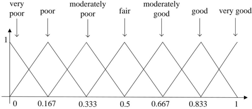
Figure 3.2: Seven-linguistic Variables with Triangular Fuzzy Membership Function ... 48
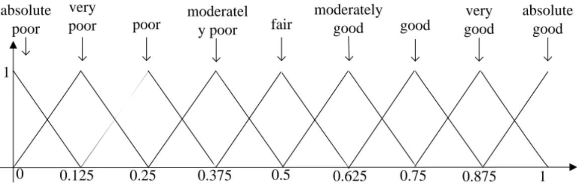
Figure 3.3: Nine-linguistic Variables with Triangular Fuzzy Membership Function ... 49
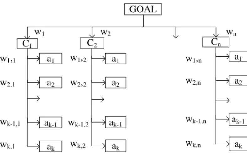
Figure 3.4: Hierarchical Structure of Decision Making Problem ... 53
Figure 3.5: FGA-TOPSIS Method ... 53
Figure 3.6: Priority Vector in Chromosome Form ... 55
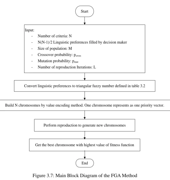
Figure 3.7: Main Block Diagram of the FGA Method ... 56
Figure 3.8: Reproduction Process ... 57
Figure 3.9: Hierarchical Structure of Restaurant's Location Decision Making ... 58
Figure 4.1: Centralized Rescue Model ... 66
Figure 4.2: Initial Process ... 67
Figure 4.3: Simulation Cycle ... 68
Figure 4.4: Node Object ... 70
Figure 4.5: Road Object ... 70
xi
Figure 4.7: Human Object ... 70
Figure 4.8: Priority in the Volunteer‟s Decision ... 71
Figure 4.9: Procedure of Task Allocation Problem ... 75
Figure 4.10: Branch on Items Based Search Tree ... 78
Figure 4.11: Example of Graph Computation (Patrick et al. 2010) ... 78
Figure 4.12: Sample GIS Map of Disaster Space... 80
Figure 4.13: Rescue Time with Proposed Model ... 81
Figure 4.14: Rescue Time with Traditional Model ... 81
Figure 4.15: Correlation between Rescue Time and Number of Link ... 82
Figure 4.16: Simulation Results with Consideration of Panic Level of Volunteer... 84
Figure 4.17: Simulation Result with Consideration of Percentage of Blocked Road Network ... 85
Figure 4.18: Simulation Result with Consideration of Percentage of High Disability Level ... 87
Figure 4.19: Simulation Result with Consideration of disconnection between Agent and Emergency Center ... 88
Figure 4.20: Simulation Result with Consideration of Number of Shelter ... 88
xii
LIST OF TABLES
Table 3.1: Converting Seven-linguistic Expressions to Triangular Fuzzy Numbers... 48
Table 3.2: Converting Nine-linguistic Expressions to Triangular Fuzzy Numbers... 48
Table 3.3: Pair-wise Comparison among Criteria ... 58
Table 3.4: Linguistic Preferences of Alternatives Respective to Each Criterion ... 59
Table 3.5: Fuzzy Number Preference of Alternatives Respective to Each Criterion ... 59
Table 3.6: Normalized Fuzzy Number Preferences ... 59
Table 3.7: Weighted Normalized Fuzzy Number Preferences ... 60
Table 4.1: Properties of Node Object ... 68
Table 4.2: Properties of Building Object ... 68
Table 4.3: Properties of Road Object ... 68
Table 4.4: Properties of Victim Agent ... 69
Table 4.5: Properties of Volunteer Agent ... 69
Table 4.6: Action of Volunteer Agent ... 69
Table 4.7: Type of Disability ... 69
Table 4.8: Pair-wise Comparison among Criteria ... 72
Table 4.9: Possible Bids ... 77
Table 4.10: Tasks Allocation and Cost after Removal of More Expensive bids ... 77
xiii
Table 4.12: Correlation between Rescue Time and Number of Link ... 81
Table 4.13: Simulation Results with Consideration of Panic Probability of Volunteer ... 83
Table 4.14: Simulation Result with Consideration of Percentage of Blocked Road Network ... 85
Table 4.15: Simulation Result with Consideration of Percentage of High Disability Level ... 86
Table 4.16: Simulation Result with Consideration of disconnection between Agent and Emergency Center ... 87
1
Chapter 1
Introduction
This chapter presents the overview, the motivation, and the objectives of the work presented in this dissertation.
1.1. Overview
The study on multi-agent based rescue simulation has been realized as an important topic recently. This study helps us to get a better understand of the rescue process in emergency situations so that the plan and preparation can be well-adapted in real cases. Rescue process is conducted under dynamic and uncertain environment so it is important to use the appropriate computer model to simulate this process.
Multi-agent based model is a good choice to study the rescue simulation because it lets us study many aspects of dynamic environments and it is very similar to real life systems. Using multi-agent based simulation, we can study how agents interact with each other. In the rescue process, the agents are rescue team, victims and emergency center. The agents make decision and perform action to reach their goal. They share the information among them in order to make decision under dynamic and uncertain environment.
In multi-agent based rescue simulation, the multi-criteria decision making and task allocation problem have been considered as a crucial topic. Each member of the rescue team will be allocated the tasks of helping victim. The problem is how to allocate the task in an appropriate way in order to save as much victims as possible. The multi-criteria decision making and task allocation problem will be more complex
2
in dynamic and uncertain environment because the agents are hard to identify in the evolution of the world. In this sense, it is very important to decide the decision making method in order to solve the task allocation problem in rescue simulation.
This dissertation addresses the challenge of designing the decision making and task allocation method in the rescue process under dynamic and fuzzy environment. Briefly, this dissertation proposes:
A multi-criteria decision making method (Fuzzy Genetic Algorithm Technique for Order Preference by Similarity to Ideal Solution: FGA-TOPSIS) for dealing with criteria and alternatives in a fuzzy environment. This method will help to calculate the weight of criteria in order to decide which volunteers should help which disabled persons.
A centralized multi-agent based rescue simulation for volunteers to help disabled people in emergency situation. The problem of which volunteer should help which disabled persons is modeled as task allocation problem and this problem is solved by using combinatorial auction mechanism.
1.2. Motivation
People with disabilities have been addressed as vulnerable population in emergency situations. The data of recent disasters i.e. Tsunami, Katrina and earthquake shows that the mortality of disabled people during the disaster were very high (Ashok Hans, 2009). The reason for this is because many handicapped people may face physical barriers or difficulties of communication that they are not able to respond effectively to crisis situations. They were not able to evacuate by themselves. Obviously, disabled people need assistances to evacuate. While in the past, persons with disabilities were not taken in consideration during the planning and mitigation
3
of disaster management, in more recent years, this group of population has been realized as a prior target to help in emergency situations. It is important to learn the needs of persons with disabilities and the various forms of disabilities in order to help them effectively and minimize the mortality.
In an emergency situation, a human tends to perform two main activities: the rescue and the evacuation. It is very difficult and costly if we want to do experiments on human rescue and or evacuation behaviors physically in real scale level. It is found that multi-agent based simulation makes it possible to simulate the human activities in rescue and evacuation process. A multi-agent based model is composed of individual units, situated in an explicit space, and provided with their own attributes and rules. This model is particularly suitable for modeling human behaviors, as human characteristics can be presented as agent behaviors. Therefore, the multi-agent based model is widely used for rescue and evacuation simulation (Ren et al. 2009, Quang et al. 2008).
The decision making in the traditional rescue models is based on static information of victims, rescue teams, and traffic condition; therefore the rescue process has difficulty to help victims effectively. Our proposed model will take advantages of wireless telecommunication to spread such information to rescue team and emergency center in order to issue appropriate decision to help people with disabilities.
The availability of multi-agent based simulation platforms has also motivated us to make simulation with multi-agent based model. We use GAMA simulation platform as test-bed for proposed methods. GAMA is an agent based, spatially explicit, modeling and simulation platform. It integrates powerful tools coming from
4
Geographic Information Systems (GIS) and Data Mining easing the modeling and analysis efforts (Taillandier et al. 2012).
1.3. Objective
The main objective is to develop a new multi-criteria decision making method and task allocation algorithms in dynamic and uncertain environment. Particularly, we apply our method on constrained environment of rescue scenarios. More specifically, this dissertation deals with the following objectives:
To apply Fuzzy Genetic Algorithm and Technique for Order Preference by Similarity to Ideal Solution to develop a new multi-criteria decision making method. This method allows calculating the important weight of criteria, and then it can be used to make decision.
To apply auction mechanism to improve the task selection among rescue agents in centralized rescue simulation model.
To use Gama simulation platform to implement the rescue simulation. This simulation platform allows working with GIS map therefore the rescue map becomes more practical.
1.4. Layout of Thesis
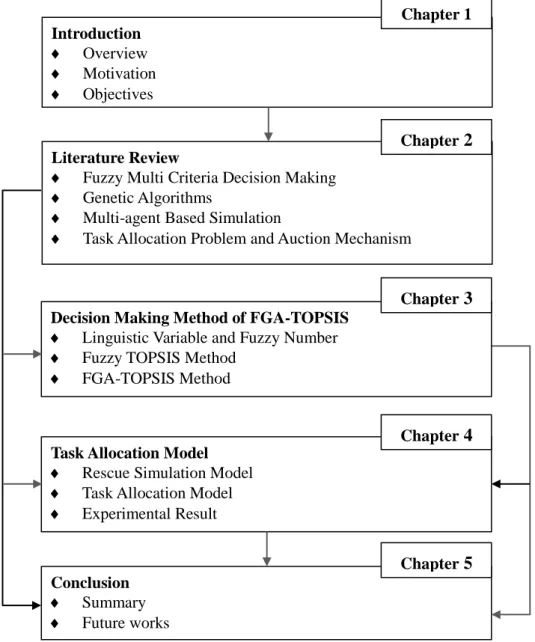
This dissertation is organized as five chapters. The structure and relation among chapters are shown in Figure 1.1.
Chapter 1 presents the introduction, motivation and objectives of this dissertation. Chapter 2 reviews the background information regarding Fuzzy system, Multi-criteria decision making, Genetic Algorithms, Multi-agent based simulation, Auction mechanism and Gama simulation platform.
5
Chapter 3 describes the new decision making method of FGA-TOPSIS (Fuzzy Genetic Algorithm-Technique for Order Preference by Similarity to Ideal Solution) with an example to clarify the procedure of this method.
Chapter 4 describes the task allocation model applied for rescue simulation by utilizing the auction mechanism. The implementation, experimentation and results of rescue simulation are also presented in this chapter.
Chapter 5 provides the summary and future research works.
Figure 1.1: Flow Chart of the Thesis Continuity
Introduction
Overview Motivation Objectives
Literature Review
Fuzzy Multi Criteria Decision Making Genetic Algorithms
Multi-agent Based Simulation
Task Allocation Problem and Auction Mechanism
Decision Making Method of FGA-TOPSIS
Linguistic Variable and Fuzzy Number Fuzzy TOPSIS Method
FGA-TOPSIS Method
Task Allocation Model
Rescue Simulation Model Task Allocation Model Experimental Result Conclusion Summary Future works Chapter 2 Chapter 1 Chapter 3 Chapter 4 Chapter 5
6
Chapter 2
Literature Review
This chapter describes the background knowledge that supports to conduct this research.
2.1. Fuzzy Multi-criteria Decision Making
"Decision making is the study of identifying and choosing alternatives based on the values and preferences of the decision maker. Making a decision implies that there are alternative choices to be considered, and in such a case we want not only to identify as many of these alternatives as possible but to choose the one that best fits with our goals, objectives, desires, values, and so on." (Harris, 1980)
Multi-criteria Decision Making (MCDM) is one of the well-known topics of Operations Research and Management Science. In a real world decision situation, the data are often imprecise and fuzzy. The classic MCDM method may have limitations to deal with imprecision or vagueness inherent in the information. For these cases, Fuzzy Multi-Criteria Decision Making methods have been developed (Kahraman, 2008). In this section, the crisp MCDM methods are first summarized briefly and then the integration of the fuzzy set theory into these methods is explained. Some recently published papers on Fuzzy MCDM are also presented.
2.1.1. Crisp Multi-criteria Decision Making
In the early 1970, Multi-criteria Decision Making (MCDM) was found as crucial field of research because it is important to make a rational decision under conflicting criteria (F. J·nos¸ 1995). A general decision making process contains eight steps shown in Figure 2.1.
7 Define problem Determine requirements Establish goals Identify alternatives Identify criteria
Select a decision making tool
Evaluate alternatives against criteria
Validate solutions against problem statement
Figure 2.1: Decision Making Process (F. J·nos¸ 1995)
Generally, a mathematical model of the MCDM can be written as follows (Waiel et al, 2008): min 𝑠 𝑍 = [𝑧1 𝑥 , 𝑧2 𝑥 , … , 𝑧𝑘 𝑥 ] 𝑇 Where: 𝑆 = {𝑥 ∈ 𝑋|𝐴𝑥 ≤ 𝑏, 𝑥 ∈ 𝑅𝑛, 𝑥 ≥ 0} Where:
Z(x) = C with x is the K-dimensional vector of objective functions and C is the vector of cost corresponding to each objective function,
S is the feasible region that is bounded by the given set of constraints, A is the matrix of technical coefficients of the left-hand side of constraints, b is the right-hand side of constraints (i.e., the available resources),
x is the n-dimensional vector of decision variables.
8
(i) Bernard Roy introduced the outranking approach and it help implementing in the Electre and Promethee methods; (ii) Keeney and Raiffa introduced the value and utility theory approaches and it help implementing in a number of methods; a special method in this branch is the Analytic Hierarchy Process (AHP) developed by Thomas L. Saaty; (iii) P.L.Yu, Stanley Zionts, Milan Zeleny, Ralph Steuer introduced the interactive multiple objective programming approach; (iv) The last branch is based on group decision and negotiation theory. It allows making decision with group dynamics and with differences in knowledge, value systems and objectives among group members (Carlsson et al., 1996).
Particularly, there are many MCDM methods which help to make decision. At this section, some of MCDM methods are described briefly as follow:
+ Pros and cons analysis is a qualitative comparison method in which good things
(pros) and bad things (cons) are identified about each alternative. Lists of the pros and cons are compared one to another for each alternative. The alternative with the strongest pros and weakest cons is preferred. It requires no mathematical skill and is easy to implement (Baker et al, 2002).
+ Maximin and maximax methods: The maximin method is based upon a strategy
that tries to avoid the worst possible performance, maximizing the minimal performing criterion. The alternative for which the score of its weakest criterion is the highest is preferred. The maximin method can be used only when all criteria are comparable so that they can be measured on a common scale, which is a limitation (Linkov et al, 2004).
+ Conjunctive and disjunctive methods: These methods require satisfactory rather
9
alternative must meet a minimal performance threshold for all criteria. The disjunctive method requires that the alternative should exceed the given threshold for at least one criterion. Any alternative that does not meet the conjunctive or disjunctive rules is deleted from the further consideration (Linkov et al., 2004).
+ Lexicographic: Using this method, attributes are rank-ordered in terms of importance. The alternative with the best performance on the most important attribute is chosen (Linkov et al., 2004).
+ Linear Assignment: This method requires, in addition to the decision matrix data, cardinal importance weights for each attribute and rankings of the alternatives with respect to each attribute.
+ TOPSIS (Technique for Order Preference by Similarity to Ideal Solution): The principle behind TOPSIS is simple: The chosen alternative should be as close to the ideal solution as possible and as far from the negative-ideal solution as possible.
+ Analytic Hierarchy Process (AHP): The analytical hierarchy process was developed primarily by Saaty (1980). The methodology of AHP is based on pair-wise comparisons of the following type 'How important is criterion 𝐶𝑖 relative to
criterion 𝐶𝑖?' Questions of this type are used to establish the weights for criteria and
similar questions are to be answered to assess the performance scores for alternatives on the subjective criteria.
However, those aforementioned MCDM methods only can be used in static environment. Actually, the data are often imprecise and fuzzy. In order to deal with imprecision and fuzziness in decision problems, Zadeh (1965) suggested applying the fuzzy set theory as a modeling tool for compensation to the limitations of crisp MCDM methods.
10 2.1.2. Fuzzy Set Theory
a. Fuzzy set
The term “fuzzy logic” was introduced when Zadeh studied on the theory of
fuzzy sets (1965). In 2005, Lee wrote a book entitled “First Course on Fuzzy Theory and Applications”. This book presents most of fundamental knowledge about fuzzy
theory. We used this book as based knowledge for studying fuzzy theory. Fuzzy sets are sets whose elements have degrees of membership. A fuzzy set A, in a universe set U, is characterized by a membership function (Figure 2.2):
𝜇 → [0, 1] 𝑤𝑒𝑟𝑒 𝜇(𝑥) 𝑖𝑛𝑑𝑖𝑐𝑎𝑡𝑒𝑠 𝑡𝑒 𝑚𝑒𝑚𝑏𝑒𝑟𝑠𝑖𝑝 𝑑𝑒𝑔𝑟𝑒𝑒 𝑜𝑓 𝑥 𝑖𝑛 𝐴, ∀𝑥 ∈ 𝑈.
Membership function 𝜇 is a mapping from each element x in A to a real number.
1 1
Fuzzy Crisp
Figure 2.2: Example of Membership Function (Yu Hen Hu, 2001)
Example of fuzzy set: There is a statement "Jenny is young". At this time, the term "young" is vague. To represent the meaning of "vague" exactly, it would be necessary to define its membership function as in Figure 2.3. When we refer "young", there might be age which lies in the range [0, 80] and we can account these "young age" in these scope as a continuous set. The horizontal axis shows age and the vertical one means the numerical value of membership function. The line shows possibility (value of membership function) of being contained in the fuzzy set "young". For example, if we follow the definition of "young" as in the figure, ten year-old boy may well be young. So the possibility for the "age ten” to join the fuzzy
11
set of "young is 1. Also that of "age twenty seven" is 0.9. But we might not say young to a person who is over sixty and the possibility of this case is 0. Now we can manipulate our last sentence to "Jenny is very young". In order to be included in the set of "very young", the age should be lowered and let us think the line is moved leftward as in the figure. If we define fuzzy set as such, only the person who is under forty years old can be included in the set of "very young". Now the possibility of twenty-seven year old man to be included in this set is 0.5.
That is, if we denote A= "young" and B="very young",
𝜇𝐴 27 = 0.9, 𝜇𝑩 27 = 0.5 1 10 20 27 30 40 50 60 0.5 0.9 Age Very young young
Figure 2.3: Fuzzy Sets Representing “Young” and “Very Young”
b. Standard Operation of Fuzzy Set
Complement: We denote the complement set of A as A. Membership degree can be
calculated as following.
𝜇𝐴 𝑥 = 1 − 𝜇𝐴 𝑥 , ∀𝑥 ∈ 𝑋
Union: Membership value of member x in the union takes the greater value of
membership between A and B.
12
Intersection of fuzzy sets A and B takes smaller value of membership function
between A and B.
𝜇𝐴∩𝐵 𝑥 = 𝑀𝑖𝑛 𝜇𝐴 𝑥 , 𝜇𝐵 𝑥 , ∀𝑥 ∈ 𝑋
c. Fuzzy Number
Fuzzy number is a fuzzy set which have the following conditions: Convex fuzzy set; Normalized fuzzy set; Its membership function is piecewise continuous; and It is defined in the real number.
Fuzzy number should be normalized and convex. Here the condition of normalization implies that maximum membership value is 1 (Figure 2.4).
∃𝑥 ∈ 𝑅, 𝜇𝐴 𝑥 = 1
The convex condition is that the line by α-𝑐𝑢𝑡 is continuous and α-cut interval
satisfies the following relation.
𝐴∝= 𝑎1 ∝ , 𝑎3 ∝
𝛽 < 𝛼 → (𝑎1 𝛽 ≤ 𝑎1 ∝ , 𝑎3 𝛽 ≥ 𝑎3 ∝ )
Figure 2.4: Fuzzy Number 𝐀 = [𝐚𝟏, 𝐚𝟐, 𝐚𝟑]
13 d. Triangular Fuzzy Number
The fuzzy sets can be presented in many ways such as triangular, trapezoidal or Gaussian. In our research we use the representation by triangular fuzzy sets. With triangular fuzzy sets A denoted by(a1, a2, a3), the triangular membership function
defined by equation (2.1) 𝐴 𝑥 = 0 𝑥 ≤ 𝑎1 𝑥 − 𝑎1 𝑎2− 𝑎1 𝑥 ∈ 𝑎1, 𝑎2 𝑎3− 𝑥 𝑎3− 𝑎2 𝑥 ∈ 𝑎2, 𝑎3 0 𝑥 ≥ 𝑎3 (2.1)
e. Operation of Triangular Fuzzy Number
Some important properties of operations on triangular fuzzy number are summarized
(1) The results from addition or subtraction between triangular fuzzy numbers result also triangular fuzzy numbers.
(2) The results from multiplication or division are not triangular fuzzy numbers.
(3) Max or min operation does not give triangular fuzzy number. But we often assume that the operational results of multiplication or division to be TFNs as approximation values.
Suppose triangular fuzzy numbers A and B are defined as
A = a1, a2, a3 B = b1, b2, b3 - Addition: A + B = a1+ b1, a2+ b2, a3+ b3
14 f. Fuzzy Number and Linguistic Variable
Linguistic variables represent crisp information in a form and precision appropriate for the problem. For example, to answer the question "What is it like outside?", one might observe "It is warm outside." Experience has shown that if it is “warm” and the time is mid-day, a jacket is unnecessary, but if it is warm and early
evening, it would be wise to take a jacket along (the day will change from warm to cool). The linguistic variables like “warm”, so common in everyday speech, convey information about our environment or an object under observation. A linguistic variable is the name of a fuzzy set. A linguistic variable encapsulates the properties of approximate or imprecise concepts in a systematic and computationally useful way. It reduces the apparent complexity of describing a system by matching a semantic tag to the underlying concept. Yet a linguistic variable always represents a fuzzy space (another way of saying that when we evaluate a linguistic variable we come up with a fuzzy set). Figure 2.5 presents the example of linguistic variable and fuzzy set (Earl Cox, 1994).
0 2 4 6 8 10 12 14 16 18
1 Long project
Figure 2.5: “Long project” Linguistic Variable and Fuzzy Set
The center of the fuzzy modeling technique is the idea of a linguistic variable. At its root, a linguistic variable is the name of a fuzzy set. In the Figure 2.5, the fuzzy set LONG is a simple linguistic variable and could be used in a rule-based system to
15
make decisions based on the length of a particular project:
if project.duration is LONG then the completion.risk is INCREASED; 2.1.3. Fuzzy Multi-criteria Decision Making
Bellman and Zadeh (1970) introduced fuzzy sets into the MCDM field. They proposed the way to solve the decision problems which are unable to solve with crisp MCDM methods. The selected alternative was defined as a point in the space of alternatives at which the membership function of a fuzzy decision attained its maximum value. To deal quantitatively with imprecision, we usually employ the concepts and techniques of probability theory. In order to apply fuzzy sets into decision making process, the differentiation between randomness and fuzziness has to be done. Essentially, randomness has to do with uncertainty concerning membership or non-membership of an object in a non-fuzzy set. Fuzziness, on the other hand, has to do with classes in which there may be grades of membership intermediate between full membership and non-membership.
The main pillar of fuzzy decision making can be summarized as follow (Bellman and Zadeh, 1970):
𝐷 = 𝐺 ∩ 𝐶
where G is the fuzzy goal, C is the fuzzy constraints, and D is the fuzzy decision that is characterized by a suitable membership function as follows:
𝜇𝐷 𝑥 = 𝑚𝑖𝑛(𝜇𝐺 𝑥 , 𝜇𝐶 𝑥 ) The maximizing decision is then defined as follows:
max
𝑥∈𝑋 𝜇𝐷 𝑥 = max𝑥∈𝑋 min(𝜇𝐺 𝑥 , 𝜇𝐶 𝑥 )
16
𝐷 = 𝐺1∩ 𝐺1∩ … ∩ 𝐺𝑘 ∩ 𝐶1∩ 𝐶2∩ … ∩ 𝐶𝑚
and the corresponding maximizing decision is written as follows: max
𝑥∈𝑋 𝜇𝐷 𝑥 = max𝑥∈𝑋 min(𝜇𝐺1 𝑥 , … , 𝜇𝐺𝑘 𝑥 , 𝜇𝐶1 𝑥 , … , 𝜇𝐶𝑚 𝑥 )
Many real-life problems have been formulated as FMCDM and have been solved by using an appropriate technique. Some of these applications involved production, manufacturing, location−allocation problems, environmental management, business, marketing, agriculture economics, machine control, engineering applications and regression modeling.
2.1.4. Researches in Fuzzy Multi-criteria Decision Making
Baas and Kwakernaak‟s (1977) proposed MCDM approach which allow rating of
criteria and ranking of multiple aspect alternatives using fuzzy sets.
Wang and Parkan (2005) investigate a MCDM problem with fuzzy preference information on alternatives and propose an eigenvector method to rank them.
Hua et al. (2005) develop a fuzzy multiple attribute decision making (FMADM) method with a three-level hierarchical decision making model to evaluate the aggregate risk for green manufacturing projects.
Ling (2006) presents a fuzzy MCDM method in which the attribute weights and decision matrix elements are fuzzy variables. Fuzzy arithmetic operations and the expected value operator of fuzzy variables are used to solve the FMCDM problem.
Xu and Chen (2007) develop an interactive method for multiple attribute group decision making in a fuzzy environment. The method can be used in situations where the information about attribute weights is partly known, the weights of decision makers are expressed in exact numerical values or triangular fuzzy numbers, and the
17
attribute values are triangular fuzzy numbers.
Recently, artificial intelligence techniques are used to solve different problems of fuzzy multi-criteria decision making. There are many researches on this aspect (Waiel, 2008).
Serafini (1985), and Ulungu et al. (1995) applied Simulated Annealing (SA) algorithm for the multi-objective framework.
Loukil et al. (2006) proposed a multi-objective SA algorithm to tackle a production scheduling problem in a flexible job-shop with particular constraints such as batch production.
Sakawa and Yauchi (1999) proposed an interactive decision-making method for solving multi-objective, non-convex programming problems with fuzzy numbers through co-evolutionary Genetic Algorithms (GA).
Sakawa and Kubota (2000) solved an application in job shop scheduling with fuzzy processing time and fuzzy due date by using GA.
Sakawa and Kato (2002) deal with the general multi-objective 0-1 programming problems that involve positive and negative coefficients. The extended GA with double strings is implemented with a new decoding algorithm for individual.
Basu (2004) applied an interactive fuzzy satisfying method based on an evolutionary programming technique for short-term multi-objective hydrothermal scheduling
2.2. Genetic Algorithms 2.2.1. Overview
There are some methods which are used to find the suitable solution in a set of solutions, for example Hill Climbing, Tabu Search, Simulated Annealing and
18
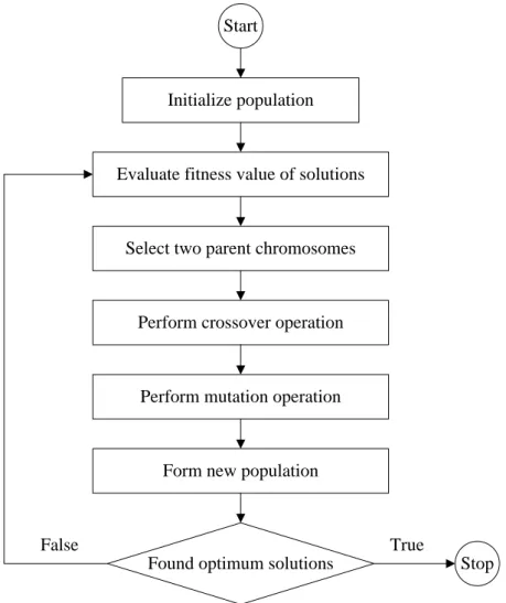
Genetic Algorithms (GA). In our research, we used GA to determine the weight of criteria in a decision making problem. Genetic algorithms were formally introduced in the United States in the 1970s by John Holland at University of Michigan. Genetic Algorithms are the heuristic search and optimization techniques that mimic the process of natural evolution. “Genetic Algorithms are good at taking large, potentially huge search spaces and navigating them, locking for optimal combinational of things, the solutions one might not otherwise find in a lifetime.” (Salvatore, 1995). Figure 2.6 show the outline of the basic Genetic Algorithm.
Start
Initialize population
Evaluate fitness value of solutions
Select two parent chromosomes
Perform crossover operation
Perform mutation operation
Form new population
Found optimum solutions Stop
True False
Figure 2.6: Outline of Basic Genetic Algorithm
19
presents a possible solution.
Step II: [Fitness] Evaluate the fitness value of each chromosome in the population. Step III: [New population] Create a new population by repeating following steps until the new population is complete.
i) [Selection] Select two parent chromosomes from a population according to their fitness. Better the fitness, the bigger chance to be selected to be the parent.
ii) [Crossover] With a crossover probability, cross over the parents to form new offspring, that is, children. If no crossover was performed, offspring is the exact copy of parents.
iii) [Mutation] With a mutation probability, mutate new offspring at each locus. iv) [Accepting] Place new offspring in the new population.
Step IV: [Replace] Use new generated population for a further run of the algorithm. Step V: [Test] If the condition is satisfied then stop, and return the best solution in current population. Otherwise go to step 2.
Actually, Genetic Algorithms are very general methods. This method will be implemented differently in various problems. In order to solve a problem with GAs, it is important to know how to generate population, chromosomes; how to select parent to perform crossover operation; how to define the fitness function.
2.2.2. Encoding of Chromosome
Before using Genetic Algorithms to solve the problem, it is important to encode potential solutions to chromosome forms so that computer can process. There are some types of encoding chromosome such as binary encoding, permutation encoding, value encoding, and tree encoding.
20 a. Binary Encoding
Every chromosome is a string of binary bits: 0 or 1. Figure 2.7 shows the example of chromosomes in binary coding.
0 0 0 1 0 0 0 1
Chromosome 1
1 1 0 0 1 0 0 1
Chromosome 1
Figure 2.7: Chromosome in Binary Coding
b. Permutation Encoding
Every chromosome is a string of numbers, which represents number in a sequence. This type of encoding is useful for ordering problem. Figure 2.8 shows the example of chromosomes in permutation coding.
1 2 4 3 7 5 8 6
Chromosome 1
5 4 1 8 7 6 2 3
Chromosome 1
Figure 2.8: Chromosome in Permutation Coding
c. Value Encoding
Every chromosome is a string of some values. Values can be in any forms such as integer numbers, real numbers, words or chars to present some complicated objects. Figure 2.9 shows the example of chromosomes in value coding.
0.1 0.2 0.4 0.3 0.7 0.5 0.8 0.6
Real number
3 2 4 1 2 1 2 4
Integer number
red green blue
Words yellow blue
21 d. Tree Encoding
It is best suited technique for evolving expressions or programs such as genetic programming. In tree encoding, every chromosome is a tree of some objects, functions or commands in programming languages. Figure 2.10 shows the example of chromosomes in tree coding.
+
x /
5 y
(+ x(/ 5y)
Figure 2.10: Chromosome in Tree Coding
2.2.3. Operator of Chromosome
Selection, crossover and mutation are three basic operators of GA. Selection is a genetic operator which is used to find the parents chromosomes to crossover and produce offspring. There are many methods of selecting parent chromosomes such as Roulette wheel, Tournament, Linear Rank, Truncation selection. Crossover is a genetic operator that combines two parent chromosomes to produce new chromosomes. The idea behind crossover is that the new chromosomes may be better than both of the parents if it takes the best characteristics from each of the parents. Crossover occurs during evolution according to a crossover probability. There many types of crossover operator: Single-point, Two-point, Uniform, Arithmetic crossover. Mutation is a genetic operator used to maintain genetic diversity from one generation of a population of chromosomes to the next. Mutation occurs during evolution according to mutation probability. Mutation is an important part of genetic search,
22
helps to prevent the population from stagnating at any local optima. There are many types of mutation such as Flip bit, Boundary, Non-Uniform, Uniform, and Gaussian.
a. Selection
+ Roulette Wheel Selection: Parents are selected according to their fitness. The
better the chromosomes are, the more chances to be selected they have. Imagine a roulette wheel where are placed all chromosomes in the population. Every chromosome has its space accordingly to its fitness value. Figure 2.11 shows the example of roulette wheel for each chromosome regarding to its fitness value.
Figure 2.11: Roulette Wheel for Chromosome
Chromosome with bigger fitness value will be selected more times. This method can be described as following steps.
[Sum] Calculate sum of all chromosome finesses in population - sum S. [Select] Generate random number R from interval (0,S)
[Loop] Go through the population and sum finesses from 0 - sum s. When the sum s is greater than r, stop and return the current added chromosome.
+ Tournament Selection: a number T of individuals is chosen randomly from the population and the best individual from this group is selected as parent. This process
Chromosome 1 Chromosome 2 Chromosome 3 Chromosome 4 Chromosome 5
23
is repeated as often as individuals must be chosen. The parameter for tournament selection is the tournament size T. T takes values ranging from 2 to N (number of individuals in population).
+ Linear Rank Selection: The chromosomes in population are ranked from 1 to N based on its fitness value. After this all the chromosomes have a chance to be selected.
+ Truncation Selection: The chromosomes are sorted according to their fitness
value. Only chromosomes its fitness value above the threshold T are selected as parents.
b. Crossover
+ Single-point Crossover: one crossover point is selected randomly. Figure 2.12 shows the example of single-point crossover operator for chromosomes in binary coding. 0 0 0 1 0 0 0 1 Parent 1 1 1 0 0 1 0 0 1 Parent 2 0 0 0 1 0 0 0 1 Offspring 1 1 1 0 0 1 0 0 1 Offspring 2 0 0 1 0 0 0 1 Parent 1 1 1 0 0 1 0 0 1 Parent 2 0 0 1 0 0 0 1 Parent 1 1 1 0 0 1 0 0 1 Parent 2
Figure 2.12: Single-point Crossover in Binary Coding
+ Two-point Crossover: two crossover points are selected, binary string from beginning of chromosome to the first crossover point is copied from one parent, the part from the first to the second crossover point is copied from the second parent and the rest is copied from the first parent. Figure 2.13 shows the example of two-point crossover operator for chromosomes in binary coding.
24 0 0 0 1 0 0 0 1 Parent 1 1 1 0 0 1 0 0 1 Parent 2 0 0 0 1 0 Offspring 1 1 1 0 0 1 Offspring 2 0 0 1 0 0 0 1 Parent 1 1 1 0 0 1 0 0 1 Parent 2 0 0 1 0 0 0 1 Parent 1 1 1 0 0 1 0 0 1 Parent 2 0 0 1 0 0 1
Figure 2.13: Two-point Crossover in Binary Coding
+ Uniform crossover: The probability of mixing ratio will control which parent will
contribute how many percentage of genes in offspring chromosomes. For example, if the mixing ratio is 0.5, then half of the genes in offspring will come from parent 1 and other half will come from parent 2. Figure 2.14 shows the example of uniform crossover operator for chromosomes in binary coding.
0 0 0 1 0 0 0 1 Parent 1 1 1 0 0 1 0 0 1 Parent 2 Offspring 1 Offspring 2 0 0 1 0 0 0 1 Parent 1 1 1 0 0 1 0 0 1 Parent 2 0 0 1 0 0 0 1 Parent 1 1 1 0 0 1 0 0 1 Parent 2 0 0 0 0 1 1 0 1 0 0 1 0 0 1 0 1
Figure 2.14: Uniform Crossover in Binary Coding
+ Arithmetic crossover: some arithmetic operations are used to make new offspring. Figure 2.15 shows the example of arithmetic crossover operator for chromosomes in binary coding.
0 0 0 1 0 0 0 1 Parent 1 1 1 0 0 1 0 0 1 Parent 2 1 1 0 0 0 0 0 1 Offspring 1 0 0 0 1 1 0 0 1 Offspring 2 OR AND
25 c. Mutation
+ Flip Bit: The mutation operator simply inverts the value of the selected genes. This type of mutation can only used for binary coding. Figure 2.16 shows the example of Flip Bit mutation for chromosome in binary coding.
1 1 0
Original offspring 1 1 0 0 1
Mutated offspring 0 1 0 1 1 1 0 1
Figure 2.16: Flip Bit Mutation in Binary Coding
+ Boundary: the mutation operator replaces the value of the selected genes with either the upper or lower bound for these genes.
+ Non-Uniform: A mutation operator that increases the probability that the amount of the mutation will be close to 0 as the generation number increases. This mutation operator keeps the population from stagnating in the early stages of the evolution then allows the genetic algorithm to fine tune the solution in the later stages of evolution. This mutation operator can only be used for integer and float genes.
+ Uniform: A mutation operator that replaces the value of the chosen gene with a uniform random value selected between the user-specified upper and lower bounds for that gene. This mutation operator can only be used for integer and float genes.
+ Gaussian: A mutation operator that adds a unit Gaussian distributed random value to the chosen gene. The new gene value is clipped if it falls outside of the user-specified lower or upper bounds for that gene. This mutation operator can only be used for integer and float genes.
26
2.3. Multi-agent based Simulation for Emergency Response
Emergency response consists of several actions which aim to reduce the damages from disaster. Basically, disaster response is a human-centric operation where humans make decisions at various levels. Information technologies (IT) plays important role in disaster response since improving the information management during the disaster. It will help in collecting information, analyzing it, sharing it, and disseminating it to the right people at the right moment (Massaguer et al., 2006). Moreover, the emergency response can be simulated by computer based model. Most computer based simulation rescue and evacuation models are based on flow model, cellular automata model, and multi-agent based model. Flow based model lacks interaction between evacuees and human behavior in crisis. Cellular automata model is arranged on a rigid grid, and interact with one another by certain rules (Ren et al., 2009). A multi-agent based model is composed of individual units, situated in an explicit space, and provided with their own attributes and rules (Quang et al., 2008). This model is particularly suitable for modeling human behaviors, as human characteristics can be presented as agent behaviors. Therefore, the multi-agent based model is widely used for rescue and evacuation simulation [Ren et al., 2009; Zaharia et al., 2011; Quang et al., 2008; Bo et al., 2009].
2.3.1. Multi-agent based Simulation
Essentially, simulations are used to virtually reproduce complex phenomena that are difficult to observe in the real world, on computers. Simulations can be divided into two classes; macroscopic and microscopic simulations according to the abstraction level of models of simulation targets. Macro simulation reproduces a phenomenon based on macroscopic viewpoint so that the whole of a simulation
27
target is represented as a single model and its behavior is defined by governing equations. Consequently, macro simulations allow observation of behaviors or changes in the overall system, but the local properties of individual elements or interactions among elements cannot be reproduced. On the other hand, micro simulation reproduces a complex social phenomenon by accumulating microscopic behaviors of models of social entities (e.g., humans or organizations) including interactions among them. Assuming that human society consists of a lot of decision-making entities, it seems natural to predict behaviors of society with a micro simulation. In particular, micro simulations manifest their ability to clearly present a variety of individual core behaviors in the reproduction and analysis of the following kinds of complex collective behavior (Ishida et al., 2010).
Basically, a multi-agent based simulation consists of three elements: agents, an environment or space, and rules (Epstein et al., 1996). Similarly, Macal and North [2010] also state that “a typical agent-based model has three elements”:
(1) A set of agents, their attributes and behaviors.
(2) The agents‟ environment: agents interact with their environment in addition to other agents.
(3) A set of agent relationships and methods of interaction: an underlying topology of connectedness defines how and with whom agents interact.
In a multi-agent based simulation model, the researcher explicitly describes the decision processes of simulated actors at the micro-level. Structures emerge at the macro level as a result of the actions of the agents, and their interactions with other agents and the environment. Three element of multi-agent based simulation will be described as follow.
28 a. Agent
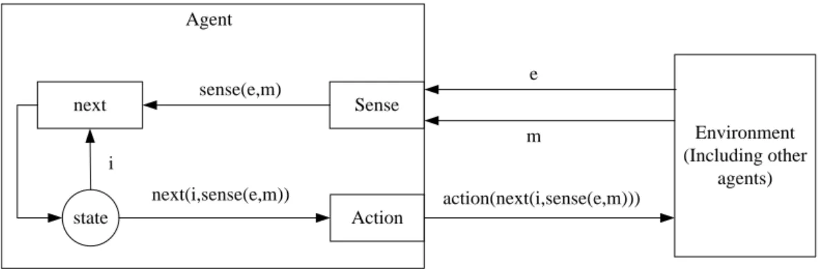
Perhaps the common feature to every definition of an agent is autonomy (Wooldridge, 2009). An agent exercises its autonomy through actions in the environment in which it is situated. An agent can perform the actions to achieve some goals or response to the changes in the environment (Wooldridge and Jennings, 1995). Furthermore, communication between agents may also take place in order to achieve shared goals. Figure 2.17 shows an abstract agent with an internal state, interacting with its environment, and with other agents situated within this environment. sense(e,m) Environment (Including other agents) next Sense Action state next(i,sense(e,m)) i e m action(next(i,sense(e,m))) Agent
Figure 2.17: Abstract Agent with State, and Its Environment (Wooldridge, 2009)
The internal state is updated via percepts, and used to determine which action to perform, via the following functions (Wooldridge , 2009):
senses: E × M → Per. The agent observes its environmental state e and receives zero
or more message(s) m from other agents, and generates a percept sense(e,m). E is the set of all possible environmental states, M is the set of all possible messages, and Per is the set of all possible percepts.
29
next: I × Per → I. The internal state i of the agent is updated via the next function,
being set to next(i,sense (e,m)). I is the set of all possible internal states, and Per is as before.
action: I → Ac. The action function programmatically represents agent behaviour. It
selects and returns an action, action(next(i,sense(e,m))), which is a member of Ac , the set of all possible actions available to the agent (which may include sending messages to other agents).
The common characteristics of an agent in the agent-based modeling community are shown as below (Macal and North, 2010):
(1) An agent is a self-contained, modular, and uniquely identifiable individual. (2) An agent is autonomous and self-directed. It has behaviours that relate
information sensed by the agent to its decisions and actions. An agent‟s information comes through interactions with other agents and with the environment.
(3) An agent has a state that varies over time. An agent‟s behaviours are conditioned on its state.
(4) An agent is social having dynamic interactions with other agents that influence its behaviour.
In emergency response simulation, an individual agent not only presents human entities such as the victim and rescuer but it also presents objects entities as well: for example, vehicles and buildings have also been modeled as agents.
b. Environment
All agents will perform actions in its environment which consider the environmental state. Therefore all entities which are relevant to an agent‟s decision
30
making, such as the buildings it observes and the road network it can travel along, should be represented in the environment, at an appropriate level of detail [Sato and Takahashi, 2011]. The environmental entities may contain attributes which can be modified to present its changes.
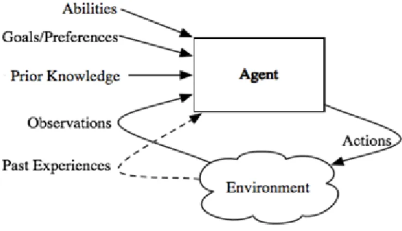
Figure 2.18 shows the interactions between an agent and its environment. Agent has abilities, goals and prior knowledge. History of interaction with the environment contains of observations of the current environment and past experiences of previous actions and observations, or other data, from which it can learn.
Figure 2.18: Agent Interacting with Environment (David and Alan 2010)
c. Interaction
There are three types of rules of behaviour for the agents and for sites of the environment (Epstein and Axtell, 1996).
(1) Agent and Environment interactions: Each agent has a repertoire of actions which it can perform in its environment. Actions are selected partly based upon what an agent senses in its environment, another form of agent-environment interaction. In order to allow the quick determination of the entities that an agent can observe,
31
environmental entities need to be stored in a data structure which provides an efficient spatial index. Also, the environment may modify an agent‟s attributes: if an agent is in a building which collapses, for example, its health attribute will deteriorate.
(2) Environment and Environment interactions: The state of the entities in the environment may evolve due to processes other than agent actions. For example, fires may spread and buildings may collapse. These processes are the environment-environment interactions.
(3) Agent and Agent interactions: Agent-agent interactions include: communication (leaders may issue instructions, trapped agents may call for help); physical contact (administration of first aid, rescue from a building); social contact (being in the proximity of someone with a contagious disease may lead to infection).
2.3.2. GAMA Simulation Platform
Many multi-agent based simulation platform exist to ease the development of an ABS (Railsback et al., 2006; Nikolai and Madey, 2007; 2009; Allan, 2010). Allan‟s review discusses 13 simulation platforms for multi-agent systems. Even if
numerous simulation platforms exist, most of the complex models are still developed from scratch. Indeed, very few platforms allow to directly work with geographical vector data (series of coordinates defining geometries) and/or to define multi-level models. Moreover, these platforms are often complex to use and their understanding can require a time investment from the modeler that can be similar to the one needed to develop a model from scratch (Patrick et al., 2012).
The GAMA agent based simulation platform provides a complete modeling and simulation development environment for building spatially explicit multi-agent
32
simulations. Its main advantages come from its versatility (domain independent) and the simplicity to define a model with it. Indeed, GAMA provides a rich, yet accessible, modeling language based on XML, that allows defining complex models integrating at the same time entities of different scales and geographical vector data (Patrick et al. 2012).
a. GAMA and Geographical Vector Data
GAMA simulation platform allows integrating geographical vector data in simulation. Geographic Information System (GIS) is used widely in large scale multi-agent based simulation. With the use of GIS data, the simulation model will be closer to the field situation. In addition, it allows using tools, like spatial analysis, coming from Geographic Information Systems (GIS) to manage these data.
GAMA simulation platform allows reading, writing of geographical data from files and/or from database. Then, the GIS becomes a simulation environment or/and background layers. The background layer allows agent moving according to this layer. For example, some agents will be able to move along a network of road, or inside a complex polygon (e.g. inside a forest represented by a polygon).
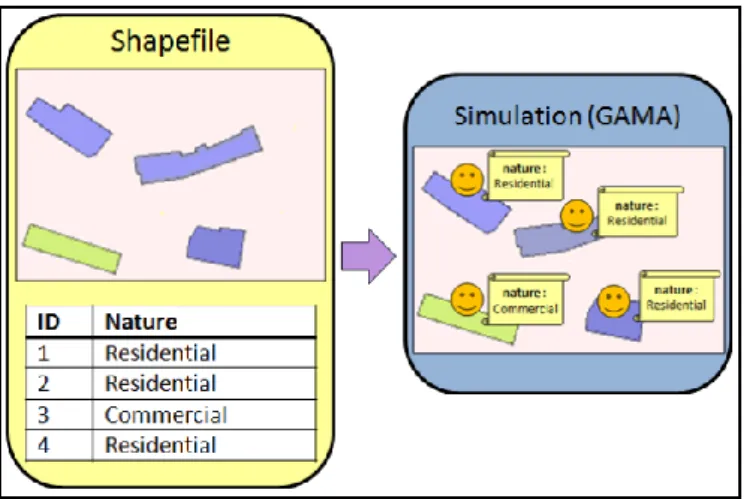
A geographical object can be considered as an agent. Thus, a road will be an agent, a building or a city, and each object contained in a geographical dataset will also be represented by an agent. The geographical object will have ability exactly like other agents in the simulation model. It is possible to give them an internal state and a behavior.
Example: From shapefile which presents building layer, the following GAML codes allow to create a set of building agents and to set the value of the attribute nature of each created building agent according to the attribute NATURE of the
33
shapefile:
<create species="building" from="shape_file_building.shp" with="[nature:: read ‘NATURE’]"/>
Figure 2.19 gives an example of converting geographical objects to agents in Gama simulation platform.
In the same way, GAMA allows to save a set of agents in a shapefile.
Example: the following GAML lines allow saving all the agents of the species building in the shapefile shape_file_building.shp and to set the value of the attribute NATURE of each geographical object according to the attribute nature of the agents:
<save species="building" to="shape_file_building.shp" with="[nature:: ‘NATURE’]"/>
GAMA also integrates several GIS features that are directly used in GAML language. These features are shown as below:
• Compute the area and the perimeter of geometry.
Example: The following GAML line allows computing the area of the geometry of the agent a:
<let name="the_area"value="a.area"/>
• Test if two geometries intersect, touch, cross, overlap each other.
Example: The following GAML lines allow to test if the geometry of the agent that is applying the action intersects the geometry geom:
<do action="interection" return="is_true"> <arg name="geometry"value="geom"/> </do>
34
Figure 2.19: Converting Geographical Objects to Agents (Patrick et al. 2012) • Compute the convex hull and the buffer geometry (Figure 2.20).
Example: The following GAML line allows computing the convex hull of the geometry of the agent that is applying the action:
<do action="convex_hull" return="result"/>
• Apply translation, rotation and scaling operations on geometry (Figure 2.21).
Example: The following GAML lines allow rotating the geometry of the agent that is applying the action with an angle of 90°:
<do action="rotation ">
<arg name="angle" value="90"/> </do>
• Compute the geometry resulting from the union, intersection or difference of two
geometries (Figure 2.22).
Example: The following GAML lines allow computing the difference between the geometry geom1 and the geometry geom2:
<do action="difference" return="result"> <arg name="geometry1" value="geom1"/>
35
<arg name="geometry2" value="geom2"/> </do>
Figure 2.20: Convex Hull and Buffer Geometry (Patrick et al. 2012)
Figure 2.21: Scaling, Rotation and Translation Geometry (Patrick et al. 2012)
Figure 2.22: Union, Intersection and Difference Actions (Patrick et al. 2012) • Compute the distance between two geometries (minimal distance).
Example: The following GAML lines allow computing the distance between the geometry of the agent that is applying the action and the geometry geom:
36
<arg name="geometry" value="geom"/> </do>
• Compute the neighborhood of an agent, i.e. all the agents that are localized at a
distance lower than a given thresholds to the agent.
Example: The following GAML lines allow computing the neighborhood of the agent ag:
<let name="neighborhood" value="ag.neighbours_geometry"/>
• Compute a random point inside geometry.
Example: The following GAML lines allow computing a random point inside the geometry geom:
<do action="place_in" return="result"> <arg name="geometry" value="geom"/> </do>
• Compute the point of a geometry that is the closest to the agent location.
Example: The following GAML lines allow computing the point of the geometry geom that is the closest to the agent that is applying the action.
<do action="closest_point_in" return="result"> <arg name="geometry" value="geom"/> </do>
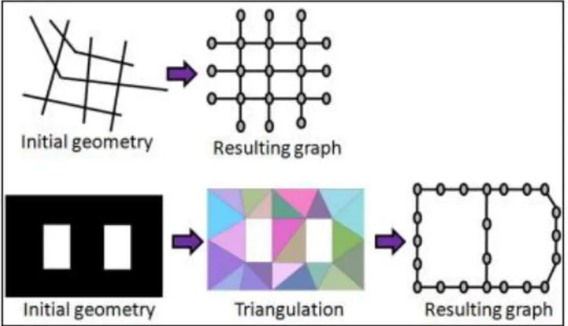
• Compute the shortest path (or the distance) inside geometry (line network or
polygon) between two points located in the geometry. For this computation, our approach consists in modeling the geometry as a graph, and in computing from it the