Mapping agricultural value chains with
international input-output data
著者
Kuroiwa Ikuo
権利
Copyrights 日本貿易振興機構(ジェトロ)アジア
経済研究所 / Institute of Developing
Economies, Japan External Trade Organization
(IDE-JETRO) http://www.ide.go.jp
journal or
publication title
IDE Discussion Paper
volume
623
year
2016-11
INSTITUTE OF DEVELOPING ECONOMIES
IDE Discussion Papers are preliminary materials circulated to stimulate discussions and critical comments
Keywords: value chain mapping, trade in value added, agricultural value chains JEL classification: C67, F14, Q17
* Executive Senior Research Fellow, Bangkok Research Centre, IDE-JETRO
IDE DISCUSSION PAPER No. 623
Mapping agricultural value chains
with international input-output data
Ikuo Kuroiwa *
November 2016
Abstract
In recent years, the analysis of trade in value added has been explored by many researchers. Although they have made important contributions by developing GVC-related indices and proposing techniques for decomposing trade data, they have not yet explored the method of value chain mapping―a core element of conventional value chain analysis. This paper introduces a method of value chain mapping that uses international input-output data and reveals both upstream and downstream transactions of goods and services induced by production activities of a specific commodity or industry. This method is subsequently applied to the agricultural value chain of three Greater Mekong Sub-region countries (i.e., Thailand, Vietnam, and Cambodia). The results show that the agricultural value chain has been increasingly internationalized, although there is still room for obtaining benefits from GVC participation, especially in a country such as Cambodia.
The Institute of Developing Economies (IDE) is a semigovernmental, nonpartisan, nonprofit research institute, founded in 1958. The Institute merged with the Japan External Trade Organization (JETRO) on July 1, 1998.
The Institute conducts basic and comprehensive studies on economic and related affairs in all developing countries and regions, including Asia, the Middle East, Africa, Latin America, Oceania, and Eastern Europe.
The views expressed in this publication are those of the author(s). Publication does not imply endorsement by the Institute of Developing Economies of any of the views expressed within.
INSTITUTE OF DEVELOPING ECONOMIES (IDE), JETRO
3-2-2, WAKABA,MIHAMA-KU,CHIBA-SHI
CHIBA 261-8545, JAPAN
©2016 by Institute of Developing Economies, JETRO
No part of this publication may be reproduced without the prior permission of the IDE-JETRO.
1
Mapping agricultural value chains with international input-output data
Ikuo Kuroiwa Bangkok Research center
Institute of Developing Economies (IDE-JETRO)
Abstract
In recent years, the analysis of trade in value added has been explored by many researchers. Although they have made important contributions by developing GVC-related indices and proposing techniques for decomposing trade data, they have not yet explored the method of value chain mapping―a core element of conventional value chain analysis. This paper introduces a method of value chain mapping that uses international input-output data and reveals both upstream and downstream transactions of goods and services induced by production activities of a specific commodity or industry. This method is subsequently applied to the agricultural value chain of three Greater Mekong Sub-region countries (i.e., Thailand, Vietnam, and Cambodia). The results show that the agricultural value chain has been increasingly internationalized, although there is still room for obtaining benefits from GVC participation, especially in a country such as Cambodia.
Keywords: value chain mapping, trade in value added, agricultural value chains Keywords: JEL classification: C67, F14, Q17
2
1. Introduction
Participation in global value chains (GVCs) has become increasingly important as a
strategy for economic development in less developed countries. Previously, the
sequence of industrial development proceeded according to a certain order, for instance,
from import to domestic production, and then to the export of manufactured goods, as
illustrated by the fundamental flying geese pattern of development (Akamatsu 1962).
Simultaneously, sequences of structural transformation occur in industries upgrading
from consumer to intermediate goods and capital goods, and from technologically
simple products to complex and sophisticated ones.
However, this sequence of industrial development has become less clear due to
the expansion of GVCs in recent decades: a currently developing country can ascend
into GVCs for sophisticated products, including high-tech products, by specializing in a
niche segment of the value chain, and become an exporter of these products apparently.
Note that such a phenomenon has occurred due to the rapid decline in trade and
communication costs, caused, in turn, by technological development and trade
liberalization. The spread of GVCs has also affected the development strategy of
developing economies. On the one hand, it is no longer necessary or efficient to build an
entire value chain from scratch through infant industry protection, as assumed in
Akamatsu’s model (Akamatsu 1962). Rather, a country can specialize in a niche
segment of the value chain, and then proceed to higher value chain activities through its
own upgrade efforts. On the other hand, globalization of the economy, spurred by trade
liberalization and economic integration, has narrowed policy space for developing
3
Against this background, trade in value added has been explored in recent years
as a method of analyzing international trade, where production processes have been
increasingly fragmented across borders and the difference between gross exports and
value added exports has grown rapidly.1 Particularly, VS (vertical specialization, that is,
foreign content in exports) and VS1 (domestic content used as input for re-export) were
originally developed by Hummels, Ishi, and Yi (2001). Moreover, Daudin, Rifflart, and
Schweisguth (2011) considered VS1* (the domestic content of import) as well. Johnson
and Noguera (2012) defined the concept of value added exports. Finally, Koopman,
Wang, and Wei (2014) synthesized these studies by tracing the value added and the
double-counted elements contained in gross exports.
However, many of these studies have focused on the structure of vertical
trade―particularly trade in intermediate inputs―and have not explored the method of the value chain mapping, which is a core element of conventional value chain analysis.
Consequently, the objective of this paper is to introduce a method of value
chain mapping using international input-output data. The major drawback of the current
value chain analysis―mainly conducted by sociologists, economic geographers, and business strategists―is the lack of objective or quantitative data. For instance, a value chain map is typically drawn using information collected via interviews or other
secondary sources. Consequently, “the analysis and policy recommendations provided
in GVC studies are often based on qualitative data and are therefore subjective”
(Frederik 2014: page 19). As shown below, the method of value chain mapping―based on Ozaki’s structural analysis―fills this void and provides objective information
1 As discussed later, trade in value added accounts for the double counting implicit in
the gross flow of trade and measures the flows of value added embodied in the trade of goods or services.
4
regarding inter-industry transactions of goods and services―as well as the creation of value added―that emerge along the value chain. Furthermore, as discussed below, the method of value chain mapping is closely related to the concept of trade in value added,
because both of them consider the value added embodied in the final output.
As an application of this method, this paper investigates the agricultural value
chains in three Greater Mekong Sub-region (GMS) countries: Thailand, Vietnam, and
Cambodia. The agricultural value chain appears to be different from that of the
manufacturing sector because it is more difficult to fragment the agricultural production
processes across space and utilize the benefits of specialization and exchange.2 However,
this opportunity can still be explored. First, modern agricultural inputs―particularly fertilizers, pesticides, and petroleum fuel―are procured from abroad, especially if countries do not have a strong industrial base. Second, agricultural products are
exported directly or indirectly as inputs for processed products. As shown below, the
agricultural value chains have been increasingly internationalized in recent decades,
although there is still room for obtaining benefits from GVC participation, especially in
a country such as Cambodia.
This paper uses OECD’s inter-country input-output (ICIO) tables for 1995 and
2011 to analyze trade in value added and quantitatively demonstrate the transformation
2 Since a great portion of agricultural value added is generated from domestic soil,
opportunities for production fragmentation across borders are limited in comparison with the machinery industry, for example. Actually, as in the mining industry, the agricultural industry has a significantly lower foreign content embodied in exports than the machinery industry. For instance, the foreign content of agriculture in Thailand, Vietnam, and Cambodia in 2011 was 0.18, 0.14, and 0.01, respectively, while that for electronics machinery was 0.65, 0.70, and 0.56, respectively (calculated from the OECD ICIO tables).
5
of the agricultural value chains in the three GMS countries.3 Furthermore, the method of
value chain mapping is applied to the ICIO tables for 2011.
The remainder of this paper is organized as follows. Section 2 introduces the
structural analysis method. Section 3, as a part of the empirical results, first compares
the structure of the agricultural sector in the three GMS countries. Subsequently, it is
followed by the results of the trade in value added analysis and the method of value
chain mapping. The results show significant differences between the three countries in
terms of the structure of agricultural value chains―particularly the usage of agricultural inputs, sourcing of foreign inputs, and access to foreign markets. Section 4 concludes
the paper with a summary of the findings.
2. Method of analysis
This section introduces the structural analysis method, originally developed by Ozaki
(1980), to investigate industrial production structure. In this paper, the structural
analysis is extended in two directions. First, Ozaki’s method, originally developed for a
single-country input-output model, is extended to a multi-country model. Second, unlike
Ozaki’s method, which considers only input structure of industry (i.e., upstream
transactions) using the Leontief inverse, the technique introduced here is also applied to
the analysis on output structure (i.e., downstream transactions) using the Ghosh inverse.
2.1 Upstream transactions
3 The OECD’s inter-country tables are available for 1995, 2000, 2005, 2008, 2009, 2010,
and 2011, from which 1995 and 2011 tables are used in this study. Additionally, it should be noted that the original ICIO tables cover 62 countries or regions, but were aggregated into 21 countries or regions, as shown in Figures 2.1–2.3. The ICIO tables cover 34 sectors, as shown in Table A1.
6
In the following, unit structure analysis is applied to multi-country input-output data to
calculate the inter-industry transactions of agricultural inputs, such as seeds, pesticides,
and fertilizers―as well as the creation of value added―directly or indirectly induced by one unit of agricultural output.
First, using an input coefficient matrix, the accounting identity on the output
side (i.e., the equality between total output and intermediate outputs plus final demand)
can be expressed as:
𝐱 = 𝐀𝐱 + 𝐟, (1) where 𝐱 = ⎣ ⎢ ⎢ ⎢ ⎡ 𝐱⋮1 𝐱𝑟 ⋮ 𝐱𝑚⎦⎥ ⎥ ⎥ ⎤
is the vector of total output (𝐱𝑟 is country 𝑟 ’s 𝑛 × 1 vector of output: m and n represent the number of countries and
sectors, respectively). 𝐀 = ⎣ ⎢ ⎢ ⎢ ⎡ 𝐀⋮11 ⋯ 𝐀⋮1𝑠 ⋯ 𝐀1𝑚⋮ 𝐀𝑟1 ⋯ 𝐀𝑟𝑠 ⋯ 𝐀𝑟𝑚 ⋮ ⋮ ⋮ 𝐀𝑚1 ⋯ 𝐀𝑚𝑠 ⋯ 𝐀𝑚𝑚⎦⎥ ⎥ ⎥ ⎤
is the multi-country input coefficient
matrix (𝐀𝑟𝑠 is an 𝑛 × 𝑛 sub-matrix that indicates the ratios of intermediate inputs
provided by industries in country 𝑟 to industries in country s relative to the
industrial outputs in country s).
𝐟 = ⎣ ⎢ ⎢ ⎢ ⎡ 𝐟⋮1 𝐟𝑠 ⋮ 𝐟𝑚⎦⎥ ⎥ ⎥
⎤ is the vector of final demand (𝐟𝑠 is
7
Solving Equation (1) for 𝑋 yields 𝐱 = (𝐈 − 𝐀)−1𝐟 = 𝐋𝐟, (2) where 𝐈 = ⎣ ⎢ ⎢ ⎢ ⎡𝐈 ⋯ 𝐎 ⋯ 𝐎⋮ ⋱ ⋮ ⋮ 𝐎 ⋯ 𝐈 ⋯ 𝐎 ⋮ ⋮ ⋱ ⋮ 𝐎 ⋯ 𝐎 ⋯ 𝐈 ⎦⎥ ⎥ ⎥
⎤ is the identity matrix (sub-matrix 𝐈 is the 𝑛 × 𝑛 identity matrix and 𝐎 represents the 𝑛 × 𝑛 matrix of zeros).
𝐋 = ⎣ ⎢ ⎢ ⎢ ⎡𝐋11⋮ ⋯ 𝐋1𝑠⋮ ⋯ 𝐋1𝑚⋮ 𝐋𝑟1 ⋯ 𝐋𝑟𝑠 ⋯ 𝐋𝑟𝑚 ⋮ ⋮ ⋮ 𝐋𝑚1 ⋯ 𝐋𝑚𝑠 ⋯ 𝐋𝑚𝑚⎦⎥ ⎥ ⎥ ⎤
is the multi-country Leontief inverse
matrix ( 𝐋𝑟𝑠 is the 𝑛 × 𝑛 Leontief inverse sub-matrix).
Then, differentiating each element in x in Equation (2) with regard to each element in f
yields
𝑙𝑖𝑖𝑟𝑠=∆𝐗𝑖𝑟
∆𝐟𝑗𝑆. (3)
In other words, the ij element of the rs sub-matrix in the Leontief inverse indicates the
output of sector i in country r, induced directly or indirectly by one unit of final demand
for sector j in country s. Thus, the column vector of sector j in country s indicates the
output of all sectors (i.e., sectors 1 through n) in all countries (i.e., countries 1 through
m), which is induced by one unit of final demand (for industry j in country s), as shown
below: 𝐥(𝒋)(𝒔) = �𝑙1𝑖1𝑠, ⋯ 𝑙𝑛𝑖1𝑠, ⋯ 𝑙1𝑖𝑟𝑠, ⋯ 𝑙𝑛𝑖𝑟𝑠, ⋯ 𝑙1𝑖𝑚𝑠, ⋯ 𝑙𝑛𝑖𝑚𝑠�′ =�∆𝐗11 ∆𝐟𝑗𝑠, ⋯ ∆𝐗𝑛1 ∆𝐟𝑗𝑠 , ⋯ ∆𝐗1𝑟 ∆𝐟𝑗𝑠, ⋯ ∆𝐗𝑛𝑟 ∆𝐟𝑗𝑠 , ⋯ ∆𝐗1𝑚 ∂∆𝐟𝑗𝑠, ⋯ ∆𝐗𝑛𝑚 ∆𝐟𝑗𝑠� ′. (4)
8
Subsequently, the unit structure for the upstream transactions can be obtained by
post-multiplying A by the diagonal matrix of column vector 𝐥(𝒋)(𝒔). 𝐔(𝒋)(𝒔)=𝐀𝐋̂(𝒔)(𝒋) = ⎣ ⎢ ⎢ ⎢ ⎡ 𝐀⋮11 ⋯ 𝐀⋮1𝑠 ⋯ 𝐀1𝑚⋮ 𝐀𝑟1 ⋯ 𝐀𝑟𝑠 ⋯ 𝐀𝑟𝑚 ⋮ ⋮ ⋮ 𝐀𝑚1 ⋯ 𝐀𝑚𝑠 ⋯ 𝐀𝑚𝑚⎦⎥ ⎥ ⎥ ⎤ ⎣ ⎢ ⎢ ⎢ ⎢ ⎢ ⎡𝐋̂(𝒔)𝟏(𝑖) ⋯ 0 ⋯ 0 ⋮ ⋱ ⋮ ⋮ 0 ⋯ 𝐋̂(𝒔)𝒓(𝑖) ⋯ 0 ⋮ ⋮ ⋱ ⋮ 0 ⋯ 0 ⋯ 𝐋̂(𝒔)𝒎 (𝒋) ⎦⎥ ⎥ ⎥ ⎥ ⎥ ⎤ , (5)
where 𝐋̂(𝒔)(𝒋) is the diagonal matrix of column vector 𝐥(𝒋)(𝒔). Then, using Equation (3), it can be shown that 𝐔(𝑖)ℎ𝑖(𝒔)𝑞𝑟 = 𝐀𝑞𝑟ℎ𝑖𝐋𝑟𝑠𝑖𝑖 =∆𝐙 ℎ𝑖
𝑞𝑟 ∆𝐱𝑖𝑟 ∆𝐱 𝑖 𝑟 ∆𝐟𝑗𝑠 = ∆𝐙 ℎ𝑖𝑞𝑟 ∆𝐟𝑗𝑠, 4
where 𝐙 ℎ𝑖𝑞𝑟 denotes the value of intermediate inputs produced by industry h in country q, and used by industry i in
country r. Hence, if j is specified as the agricultural sector, 𝐔(𝑖)ℎ𝑖(𝒔)𝑞𝑟represents a transaction of inputs from industry h in country q to industry i in country r, which is
induced by one unit of final demand for the agricultural products in country s. Then,
𝐔(𝑖)(𝒔) indicates the sequences of inter-industry transactions of goods and services that
occur along the upstream agricultural value chain.
Similarly, induced value added—actually paid as remuneration for primary
inputs, such as labor compensation, profits, and taxes—is calculated by
post-multiplying the row vector of the value added coefficients by 𝐋̂(𝒔)(𝒋). 𝐯(𝒋)(𝒔)′=𝐯′𝐋̂
(𝒋) (𝒔)
4 Due to the assumption of linearity in the input-output model, it holds that 𝐀
ℎ𝑖 𝑞𝑟=𝐙 ℎ𝑖𝑞𝑟
𝐱𝑖𝑟 =
∆𝐙 ℎ𝑖𝑞𝑟 ∆𝐱𝑖𝑟.
9 = [𝐯1′ ⋯ 𝐯𝑟′ ⋯ 𝐯𝑚′] ⎣ ⎢ ⎢ ⎢ ⎢ ⎢ ⎡𝐋̂(𝒔)𝟏(𝑖) ⋯ 0 ⋯ 0 ⋮ ⋱ ⋮ ⋮ 0 ⋯ 𝐋̂(𝒔)𝒓(𝑖) ⋯ 0 ⋮ ⋮ ⋱ ⋮ 0 ⋯ 0 ⋯ 𝐋̂(𝒔)𝒎 (𝒋) ⎦⎥ ⎥ ⎥ ⎥ ⎥ ⎤ , (6) where 𝐯 = ⎣ ⎢ ⎢ ⎢ ⎡ 𝐯⋮1 𝐯𝑟 ⋮ 𝐯𝑚⎦⎥ ⎥ ⎥
⎤ is a column vector of the value added coefficients5 (𝐯𝑟 is country 𝑟 ’s 𝑛 × 1 vector of the value added coefficients).
Here, similar to Equation (5), it holds that 𝐯(𝑖)𝑖(𝑠)𝑟 = 𝐯𝑖𝑟𝐋𝑟𝑠𝑖𝑖 = ∆𝐯𝑖 𝑟 ∆𝐱𝑖𝑟 ∆𝐱 𝑖𝑟 ∆𝐟𝑗𝑠 = ∆𝐯𝑖𝑟 ∆𝐟𝑗𝑠, (7)
where 𝐯𝑖𝑟 denotes the value added for industry i in country r. Hence, if j is specified as the agricultural sector, 𝐯(𝑖)𝑖(𝑠)𝑟 represents the value added in industry i in country r required to produce one unit of the agricultural products in country s.
Furthermore, it should be noted that 𝐯(𝑖)𝑖(𝑠)𝑟 (r ≠ s) represents the value added exports produced by industry i in source country r and absorbed by industry j in destination country s.6
It is also important to note that the sum of row 𝐯(𝒋)(𝒔)′ in Equation (6) always equals one, because of the equality between exogenously given final demand―one unit of final demand for sector j in country s―and the sum of value added generated endogenously in all sectors of all countries or regions.
2.2 Downstream transactions
For mapping downstream transactions, a different approach is necessary. This paper
proposes to use the Ghosh inverse (Ghosh 1958) as an alternative to the Leontief
5 A value added coefficient is the ratio of value added to total output.
10
inverse. As a mirror image of the Leontief inverse, the Ghosh inverse indicates output in
the respective sectors induced by one unit of primary inputs for a specific sector7.
Using the allocation coefficient matrix, the accounting identity on the input
side (i.e., the equality between total inputs and intermediate inputs plus value added) is
expressed as 𝐱′= 𝐱′𝐁 + 𝐯′, (8) where 𝐁 = ⎣ ⎢ ⎢ ⎢ ⎡ 𝐁⋮11 ⋯ 𝐁⋮1𝑠 ⋯ 𝐁1𝑚⋮ 𝐁𝑟1 ⋯ 𝐁𝑟𝑠 ⋯ 𝐁𝑟𝑚 ⋮ ⋮ ⋮ 𝐁𝑚1 ⋯ 𝐁𝑚𝑠 ⋯ 𝐁𝑚𝑚⎦⎥ ⎥ ⎥ ⎤
is the multi-country output coefficient
matrix (𝐁𝑟𝑠 is the 𝑛 × 𝑛 sub-matrix that indicates the ratio of intermediate outputs
distributed by the industries in country 𝑟 to the industries in country 𝑠 relative to the industrial outputs in country r).
𝐯 = ⎣ ⎢ ⎢ ⎢ ⎡ 𝐯⋮1 𝐯𝑟 ⋮ 𝐯𝑚⎦⎥ ⎥ ⎥ ⎤ :
is the vector of value added (𝐯𝑟 is country 𝑟’s 𝑛 × 1 vector of value added).
Solving Equation (8) for x gives 𝐱′= 𝐯′(𝐈 − 𝐁)−1= 𝐯′𝐆, (9) where 𝐆 = ⎣ ⎢ ⎢ ⎢ ⎢ ⎡𝐆11 ⋯ 𝐆1𝑠 ⋯ 𝐆1𝑚 ⋮ ⋮ ⋮ 𝐆𝑟1 ⋯ 𝐆𝑟𝑠 ⋯ 𝐆𝑟𝑚 ⋮ ⋮ ⋮ 𝐆𝑚1 ⋯ 𝐆𝑚𝑠 ⋯ 𝐆𝑚𝑚⎦⎥ ⎥ ⎥ ⎥
⎤ is the multi-country Ghosh inverse matrix (𝐆𝑟𝑠 is the 𝑛 × 𝑛 Ghosh inverse sub-matrix).
7 For the repercussion mechanism of the Ghosh model, see Chapter 12 in Miller and
11
Then, differentiating each element in x in Equation (8) with regard to each element in v
yields
𝑔𝑖𝑖𝑟𝑠=∆𝐗𝑗𝑠
∆𝐯𝑖𝑟 . (10)
It should be noted that, contrary to Equation (3), 𝑔𝑖𝑖𝑟𝑠 represents the output of sector j in country s, induced directly or indirectly by one unit of primary inputs (i.e., primary
inputs whose total remuneration adds up to one unit of value added) in sector i in
country r. Therefore, the row vector of sector i in country r reveals the output of all
sectors in all countries, induced by sector i in country r:
𝐠(𝒊)(𝒓) = [𝑔𝑖1𝑟1, ⋯ 𝑔𝑖𝑛𝑟1, ⋯ 𝑔𝑖1𝑟𝑠, ⋯ 𝑔𝑖𝑛𝑟𝑠, ⋯ 𝑔𝑖1𝑟𝑚, ⋯ 𝑔𝑖𝑛𝑟𝑚] =�∆𝐗11 ∆𝐯𝑖𝑟, ⋯ ∆𝐗𝑛1 ∆𝐯𝑖𝑟, ⋯ ∆𝐗1𝑠 ∆𝐯𝑖𝑟, ⋯ ∆𝐗𝑛𝑠 ∆𝐯𝑖𝑟, ⋯ ∆𝐗1𝑚 ∆𝐯𝑖𝑟 , ⋯ ∆𝐗𝑛𝑚 ∆𝐯𝑖𝑟�. (11)
Then, the unit structure for the downstream transactions can be obtained by
pre-multiplying B by the diagonal matrix of row vector 𝐠(𝑖)(𝑟). 𝐃(𝒊)(𝒓)=𝐆�(𝒊)(𝒓)𝐁 = ⎣ ⎢ ⎢ ⎢ ⎢ ⎢ ⎡𝐆�(𝒊)(𝑟)1 ⋯ 0 ⋯ 0 ⋮ ⋱ ⋮ ⋮ 0 ⋯ 𝐆�(𝒊)(𝑟)𝑠 ⋯ 0 ⋮ ⋮ ⋱ ⋮ 0 ⋯ 0 ⋯ 𝐆�(𝒊)(𝑟)𝑚⎦⎥ ⎥ ⎥ ⎥ ⎥ ⎤ ⎣ ⎢ ⎢ ⎢ ⎡ 𝐁⋮11 ⋯ 𝐁⋮1𝑠 ⋯ 𝐁1𝑚⋮ 𝐁𝑟1 ⋯ 𝐁𝑟𝑠 ⋯ 𝐁𝑟𝑚 ⋮ ⋮ ⋮ 𝐁𝑚1 ⋯ 𝐁𝑚𝑠 ⋯ 𝐁𝑚𝑚⎦⎥ ⎥ ⎥ ⎤ , (12)
where 𝐆�(𝒊)(𝒓) is the diagonal matrix of row vector 𝐠(𝒊)(𝒓). Note that, similar to Equation (5), it holds that 𝐃(𝒊) 𝒋𝒋(𝒓) 𝒔𝒔 = 𝐆𝑖𝑖𝑟𝑠𝐁𝑖𝑗𝑠𝑠= ∆𝐱 𝑗 𝑠 ∆𝐯𝑖𝑟 ∆𝐙 𝑗𝑗𝑠𝑠 ∆𝐱𝑗𝑠 = ∆𝐙 𝑗𝑗𝑠𝑠
∆𝐯𝑖𝑟 . Thus, if i is specified as the
agricultural sector, 𝐃(𝒊)(𝒓) indicates sequences of inter-industry transactions of goods and services that occur along the downstream agricultural value chain in country r.
12
Similarly, the final demand induced by agricultural value added is calculated
as: 𝐅(𝒊)(𝒓)=𝐆�(𝒊)(𝒓)𝐅 = ⎣ ⎢ ⎢ ⎢ ⎢ ⎢ ⎡𝐆�(𝒊)(𝑟)1 ⋯ 0 ⋯ 0 ⋮ ⋱ ⋮ ⋮ 0 ⋯ 𝐆�(𝒊)(𝑟)𝑠 ⋯ 0 ⋮ ⋮ ⋱ ⋮ 0 ⋯ 0 ⋯ 𝐆�(𝒊)(𝑟)𝑚⎦⎥ ⎥ ⎥ ⎥ ⎥ ⎤ ⎣ ⎢ ⎢ ⎢ ⎡ 𝐅⋮1 𝐅𝑠 ⋮ 𝐅𝑚⎦⎥ ⎥ ⎥ ⎤ , (13) where 𝐅 = ⎣ ⎢ ⎢ ⎢ ⎡ 𝐅⋮1 𝐅𝑠 ⋮ 𝐅𝑚⎦⎥ ⎥ ⎥ ⎤ :
is the matrix of the final demand
coefficient,8 (𝐅𝑟 is country 𝑟 ’s 𝑛 × 6 sub-matrix of the final demand coefficients).9
It should be noted that, similar to Equation (6), the sum of all matrix elements
in 𝐅(𝒊)(𝒓) in Equation (13) always equals one because of the equality between
exogenously given value added―one unit of value added (or primary inputs) for sector i in country r―and the sum of final demand (or final outputs) endogenously generated in all sectors for all countries or regions.
3. Empirical results
3.1 The structure of the agricultural sector
8 A final demand coefficient is the ratio of final demand to total output.
9 The reason that the final demand matrix for each country has 6 x 𝑚 columns is that,
in the ICIO tables, the distribution of goods and services for final consumption is divided into 𝑚 destination countries and six final demand columns (i.e., household consumption, non-profit institutions serving households, general government final consumption, gross fixed capital formation, changes in inventories, and direct purchases abroad by residents) for each destination country.
13
In this section, agricultural value chains are discussed from the viewpoint of production
and trade structure. It should be noted that the three countries―Thailand, Vietnam, and Cambodia―are in different stages of industrial development and, thus, their agricultural value chains can be situated in different positions with regard to the regional production
networks.
Table 1 compares the agricultural sector in the three countries in terms of the
shares of agricultural value added, exports, and the degree of diversification in the
industrial structure.10 During 1995–2011, the agricultural sector grew rapidly in these
three countries, with Thailand generating the largest value added, followed by Vietnam
and Cambodia. During the same period, the share of agricultural value added declined,
with the exception of Thailand, and the diversification of industrial structure increased
in all countries, as reflected by a decrease in the Herfindahl index.11 However, it should
be noted that the agricultural sector still occupies a relatively high value added share,
although a higher income country tends to register a lower share.
- Table 1 -
During 1995–2011, agricultural exports also increased sharply in Thailand and
Vietnam, but declined slightly in Cambodia. Correspondingly, the share of agricultural
exports increased in Thailand and Vietnam, but declined sharply in Cambodia, with a
slight decrease in export diversification. It should be noted, however, that Cambodia’s
10 In the OECD ICIO tables, the agricultural sector is actually composed of agriculture,
hunting, forestry, and fishing (see Table A1 in Appendix 1).
11 The Herfindahl index is calculated as 𝐻𝑠= ∑ �𝜆 𝑖 𝑆�, 𝑛
𝑖=1 where 𝜆𝑖𝑆 is the value added
(or exports) share of sector i in country S, and n is the number of industrial sectors in country S.
14
export structure was unconventional in the sense that the share of textile products and
footwear had increased drastically, achieving 40 percent of total exports in 2011, thus
reducing the share occupied by the other sectors, including the agricultural sector.
Regarding the export orientation of the agricultural sector, Thailand and
Vietnam increased their export dependency, their ratio of exports to value added
reaching 29.6 percent and 24.1 percent, respectively, in 2011; on the other hand,
Cambodia’s export ratio was 4.7 percent in 2011.12
3.2 Trade in value added: VS share
Figure 1 shows the VS share of the agricultural sector for 21 countries or regions. The
VS share of the agricultural sector represents the percentage share of foreign value
added that is embodied in agricultural exports (i.e., the share of value added that is
induced by agricultural exports, but accrues to foreign countries).13
Figure 1 shows that in all countries or regions, except New Zealand, the VS
share increased significantly during 1995–2011. This demonstrates that these countries
increased their dependency on imported agricultural inputs, such as fertilizers and
pesticides. Among the three countries, Thailand had the highest VS share, followed by
Vietnam. On the other hand, Cambodia had an extremely low VS share, lower than
some large countries, such as China, Indonesia, and India. This implies that the
agricultural value chain in Cambodia was highly self-sufficient with little dependency
on foreign inputs. From the viewpoint of a value chain, it can be said that Cambodia
12 It should also be noted that Cambodia’s agricultural exports could be seriously
underestimated due to unofficial export of agricultural products―such as paddy, cassava, and maize―to Vietnam and Thailand.
13 For details on the VS share and the method of decomposition introduced in this paper,
15
was not fully utilizing opportunities to improve productivity by participating in GVCs.
It should be noted that engagement with GVCs can increase productivity by facilitating
access to cheaper or higher-quality inputs.14 It is particularly relevant in a country such
as Cambodia, where procurement of high-quality agricultural inputs is severely
constrained by underdeveloped manufacturing sectors.
-Figure 1-
Figures 2.1 to 2.3 breakdown the VS share into the country of origin, where the
foreign value added is created by the agricultural exports of the three countries. It is
notable that, among the three countries, China’s share increased remarkably, suggesting
that it has become an important supplier of agricultural inputs for these countries. It is
also worth noting that, along with the major exporters of agricultural inputs―such as China, the EU, the USA, and the rest of the world (ROW)―Vietnam and Thailand became important suppliers of agricultural inputs to Cambodia.
-Figures 2.1, 2.2, 2.3-
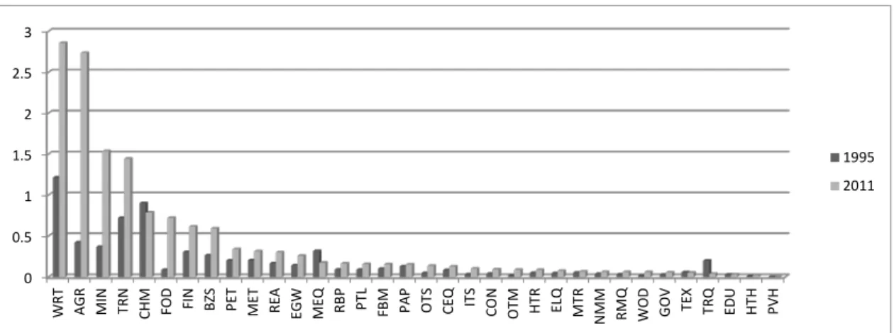
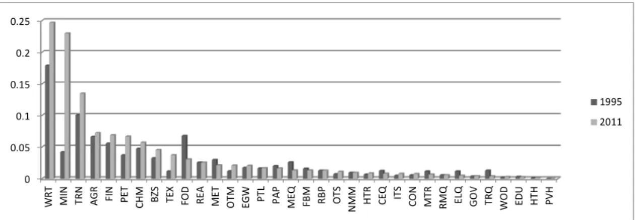
Figures 3.1 to 3.3 breakdown the VS share into the sector of origin, where the
foreign value added is generated by agricultural exports. In Thailand, the share of the
14 It is shown that an industry with a high share of imported inputs displays, on
average, higher productivity among OECD countries, because foreign inputs embody more productive technology, and resources are re-allocated more efficiently. Particularly, increased productivity results from: (1) a price effect—increased intermediate imports result in stronger competition and therefore lower prices for inputs; (2) a supply effect—increased imports enhance the variety of inputs available; (3) a productivity effect: new intermediate inputs may spur innovation in the final goods sector by enhancing access to knowledge (OECD 2013).
16
foreign content was high for minerals, chemicals, agriculture, food products, and refined
petroleum. Additionally, the service sectors, such as wholesale and retail trade, financial
intermediation, transport, and business services, showed high foreign content share. It
should be noted that these sectors were ranked highly in Vietnam and Cambodia as well,
reflecting similarity in terms of imported inputs.
-Figures 3.1, 3.2, 3.3-
3.3 Mapping the value chain
The VS indicates the share of foreign content embodied in exports. Furthermore, the
decomposition of the VS is useful to trace the source country and industry of the foreign
content. However, since these are aggregate data, they cannot provide sufficient
information to trace value added activities along the chain. Furthermore, unlike the
conventional value chain analysis, trade in value added does not provide any
information regarding the transactions of goods and services that accompany
value-added activities. However, the method of value chain mapping discussed below
takes into account these constraints.
(1) Upstream transactions
The unit structure analysis provides information regarding the flow of goods and
services transactions, as well as the creation of value added, which is induced by one
unit of final demand for a specific sector. Using the above information, a value chain is
17
For instance, Figures 4.1, 4.2, and 4.3 are respectively constructed based on the
inter-industry transactions in Tables A2.1, A2.2, and A2.3 (Appendix 3). The direction
of the arrows in Figure 4.1 indicates which inputs (shown on the left-hand side of the
arrows) are used to produce which outputs (shown on the right-hand side), with the final
destination of the arrows being one unit of an agricultural product. In summary, these
figures demonstrate the sequence of upstream transactions of goods and services,
induced by one unit of agricultural products. Additionally, it should be noted that the
value added activities that accompany the transactions of goods and services are
recorded by the corresponding sectors under the VA row in Tables A2.1, A2.2, and A2.3.
For instance, Figure 4.1 shows that inputs from FOD (1.4) and AGR (2.9) were used to
produce FOD outputs in Thailand (the figures in the parenthesis are derived from Table
A2.1). Simultaneously, it is demonstrated that value added (2.8) was generated in the
FOD sector in this production process. -
- Figure 4.1, Figure 4.2 and Figure 4.3 -
Figure 4.1 shows that, in 2011, the Thai agricultural sector received inputs from
refined petroleum, chemicals, rubber, food products, and agriculture. Additionally, it
had service inputs from the wholesale and retail trade, transport, and financial
intermediation (for the volume of inter-industry transactions and the value added
generated, see Table A2.1). Among them, a value chain sequence, minerals → refined petroleum → agriculture, can be seen in both the domestic and foreign inputs. Because a higher consumption of refined petroleum is considered to reflect a higher usage of
18
agricultural machinery―such as tractors and harvesters―the existence of such a sequence reflects a higher level of mechanization in the Thai agricultural sector.
Moreover, since chemical products, which include chemical fertilizers and
pesticides, are critical inputs for agriculture, the sequence of chemicals → agriculture, is an important segment of the agricultural value chain, for which the major suppliers of
chemicals were Thailand, Japan, China, and the ROW.
Figure 4.2 shows significant similarities in the structure of the value chains
between Vietnam and Thailand, but a notable difference is that chemical inputs were
relatively low in Vietnam (see Tables A2.1 and A2.2). Furthermore, unlike Thailand,
inputs from refined petroleum do not appear in Figure 4.2. Regarding foreign inputs,
inputs from food products, agriculture, and wholesale and retail trade were relatively
high, but neither chemicals nor refined petroleum were included in this category. These
results suggest that there is still room for improving the productivity of Vietnam’s
agricultural sector in terms of usage of chemicals and agricultural machinery,
particularly those imported.
The above structure is more clearly demonstrated in Figure 4.3. As shown in
Table A2.3, Cambodia had an extremely high value added share of the agricultural
sector (98.14). This implies that Cambodia’s agricultural sector was highly
self-sufficient and its backward linkage with other sectors, including chemical inputs
and refined petroleum, was extremely weak. As in other countries, a variety of
19
is strikingly small.15 However, it is notable that refined petroleum imported from
Vietnam was used by the Cambodian agricultural sector.
(2) Downstream transactions
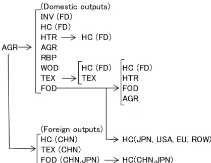
Figures 5.1, 5.2, and 5.3 are produced based on Tables A3.1, A3.2, and A3.3
respectively. Unlike Figure 4.1, Figure 5.1 starts with one unit of an agricultural output,
used as an intermediate input for other sectors, such as food products. The outputs of the
other sectors are subsequently used as inputs and stimulate the outputs of other sectors
such as hotels and restaurants. Consequently, these figures demonstrate the sequence of
downstream transactions of goods and services induced by one unit of an agricultural
output.
- Figure 5.1, Figure 5.2 and Figure 5.3 -
Figure 5.1, shows that Thai agricultural outputs were used as intermediate
inputs for the manufacturing sectors, such as food products, rubber products, wood
products, and textiles. Among them, food products received the largest amount of inputs
from agriculture (35.6 units; see Table A3.1). Then, the food products were consumed
by other sectors, including household consumption in Thailand, Japan, the USA, the EU,
and the ROW. Hotels and restaurants, whose services were finally consumed by
households, were an important sales destination for agricultural outputs.
15 Regarding agricultural inputs in Cambodia, a government official whom the author
met at the Ministry of Agriculture, Forestry, and Fisheries (MAFF) appreciated that “chemicals used in agriculture are too little because of higher prices of agricultural chemicals imported from abroad and traditional farming systems, where the main purpose of farming is for household-consumption.”
20
Some agricultural outputs were exported to China and Japan. Food products
produced using agricultural outputs from Thailand were consumed by households in
these countries (see the right hand side of Table A3.1).
Figure 5.2 shows that the basic structure of Vietnam’s agricultural value chain
is similar to that of Thailand. Particularly, similar to Thailand, Vietnam’s food products
were stimulated strongly by agricultural outputs (41.9 units; see Table A3.2), and the
sectors that used food products as inputs were also similar to Thailand’s. In Vietnam,
however, household consumption in the EU played a more important role as a
destination for Vietnam’s food products.
In Cambodia, transactions of goods and services induced by a unit of
agricultural output were significantly small (see Figure 5.3 and Table A3.3). First, this
reflects the nature of the Cambodian agricultural sector, where a large percentage of
agricultural output was consumed by domestic households; thus, its forward linkage
with other sectors was extremely weak.16 Second, unlike Thailand and Vietnam,
Cambodia’s food products had no significant impact on household consumption abroad.
This is because Cambodia’s food processing industry is underdeveloped, and the bulk of
agricultural products were exported directly without processing.
Third, part of hotels and restaurants services, which had inputs from the
agricultural sector, were consumed by direct purchase by residents from the USA. This
reflects the fact that Cambodia attracted a large number of foreign tourists, who spent
large amounts of money at hotels and restaurants in Cambodia. Finally, it is worth
noting that neighboring countries were becoming important trade partners of Cambodia;
for instance, a significant amount of Cambodia’s agricultural output was exported to
16 As previously discussed, Cambodia’s external linkages could be significantly
21
Vietnam, thus stimulated the output of food products here. However, this implies that
potentially lucrative markets, such as the EU, the USA, Japan, China, and Korea, have
not been fully exploited by Cambodian producers yet.
4. Conclusion
This paper introduced a method of the value chain mapping that uses international
input-output data. The international input-output tables are one of the most reliable data
sources that document the transactions of goods and services across borders. Therefore,
this method combines the concept of value chain mapping with the technique of
input-output analysis. The method clearly demonstrates that the value chain of a specific
sector or commodity can be mapped with both upstream and downstream transactions
of goods and services along the chain. Furthermore, the method provides more detailed
information regarding the sequences of the value added activities along the chain than
does analysis of trade in value added.
The result of the analysis shows that Thailand’s agricultural value chains are
the most advanced and internationalized among the three countries. Particularly, critical
agricultural inputs, such as chemicals and refined petroleum, were procured from both
international and domestic sources. On the other hand, Vietnam and Cambodia were not
fully utilizing opportunities to improve productivity by participating in GVCs.
Specifically, Cambodia’s agricultural sector was highly self-sufficient with little
dependency on imported inputs. Conversely, Thailand and Vietnam show rather
diversified downstream transactions. In particular, food products produced using
agricultural outputs were widely consumed by households in both domestic and
22
sales destinations of agricultural outputs. In Cambodia, the transactions of goods and
services stimulated by agricultural production were significantly smaller. Moreover,
Cambodia’s food products had no significant impact on household consumption abroad,
due to the underdevelopment of the food processing industry in Cambodia.
Although the method proves useful, there are some constraints regarding the
data and methodology. First, it is desirable to construct more disaggregated data with a
greater number of sector classifications, particularly for agriculture and related
industries. Second, the current input-output data has an industrial activity-based sector
classification, while a conventional value chain analysis concerns business
functions―such as design, production, marketing, distribution, and support to the final consumer―performed by each firm. Therefore, this difference needs to be reconciled so that input-output analysis can be performed more in line with the concept of the value
chain analysis. Finally, it is important to improve trade statistics, especially for a
country such as Cambodia, whose trade statistics could be underestimated due to
23
References
Akamatsu, Kaname. 1962, “Historical pattern of economic growth in developing countries.” The Developing Economies 1: 3-25.
Daudin, Guillaume, Christine Rifflart, and Danielle Schweisguth. 2011. “Who Produces for Whom in the World Economy” Canadian Journal of Economics 44 (4): 1403-37.
Frederick, Stacey. “Combining the Global Value Chain and global I-O approaches”, a
paper presented at the International Conference on the Measurement of International Trade and Economic Globalisation, Aguascalientes, Mexico,
29 September – 1 October 2014.
Gosh, Ambica. 1958. “Input-Output Approach to an Allocation System.” Econometrica 25: 58-64.
Hummels, David, Jun Ishii, and Kei-Mu Yi. 2001. “The nature and growth of vertical specialisation in world trade.” Journal of International Economics 54: 75-96.
Johnson, Robert C., and Guillermo Noguera. 2012. “Accounting for Intermediates: Production Sharing and Trade in Value Added.” Journal of International
Economics 86 (2): 224-36.
Koopman, Robert, Zhi Wang, and Shag-Jin Wei. 2014. “Tracing Value Added and Double Counting of Gross Exports.” American Economic Review, 104 (2):459-494.
Miller, Ronald E., and Peter D. Blair. 2009. Input-Output Analysis: Foundation and
Extensions, Second Edition. Cambridge University Press: New York.
OECD. 2013. "Interconnected Economies: Benefitting from the Global Value Chains.”
Synthesis Report. http://www.oecd.org/sti/ind/interconnected-economies- GVCs-synthesis.pdf (downloaded on 25 October, 2015).
Ozaki, Iwao. 1980. “Structural Analysis of Economic Development (3): Determination of the Basic Structure of the Economy (in Japanese) Keizai Hatten of Kouzou Bunseki (3): Keizai no Kihonteki, Kouzou of Kettei.” Keio Journal
24
Appendix 1: Sectoral classification of OECD ICIO tables
The following table shows the sectoral classification of the OECD ICIO tables.
25
Appendix 2: The VS share and its decomposition
The VS share represents the percentage share of foreign content embodied in exports,
i.e., the share of value added induced by exports but accrued to foreign countries. The
methodology was originally developed by Hummels, Ishi, and Yi (2001), and it was
introduced into the analysis of trade in value added by Koopmans, Wang, and Wei
(2014).
Using Equation (7) in Section 2.1, the VS share of sector j in country s
(Equation (40) in Koopmans, Wang, and Wei, 2014) can be expressed as:
𝑉𝑉(𝑖)(𝑠) share=100 X ∑𝑟≠𝑠𝑚 ∑𝑛𝑖=1𝐯𝑖𝑟𝐋𝑟𝑠𝑖𝑖 = 100 X ∑𝑚𝑟≠𝑠∑𝑛𝑖=1𝐯(𝑖)𝑖(𝑠)𝑟, (a1)
where 𝐯(𝑖)𝑖(𝑠)𝑟 represents the value added in sector i in country r that is induced by one unit of final demand for sector j in country s.17 Here, the VS share is expressed in
percentage terms, so that it can range from 0 to 100.18 Furthermore, the 𝑉𝑉(𝑖)(𝑠) share can be decomposed as follows.
(1) Share of foreign content by country of origin
17 Note that, in the input-output framework, the induced output or value added is
identical regardless of whether it is induced by exports or other final demand items.
18 It should also be noted that, as a mirror image of the 𝑉𝑉
(𝑖)(𝑠) share, a measure of
vertical specialization can be calculated using the Ghosh inverse as follows:
𝑉𝑉(𝐺)(𝑖)(𝑟) share=100 X ∑𝑠≠𝑟𝑚 ∑𝑖=1𝑛 𝐆𝑟𝑠𝑖𝑖 𝑓𝑖𝑠, where 𝑓𝑖𝑠 indicates the final demand coefficient
for sector j in country s. Therefore, the 𝑉𝑉(𝐺)(𝑖)(𝑟) share indicates the share of the final
outputs produced by foreign producers when one unit of value added is generated by sector i in country r. Theoretically, the 𝑉𝑉(𝐺)(𝑖)(𝑟) can be a sector-level counterpart for VS1, which measures the value of the exported goods used as imported inputs by other countries to produce their exports―this, in turn, indicates the strength of forward linkages across countries. Actually, as in VS1 in Koopman, Wang, and Wei (2014), the 𝑉𝑉(𝐺)(𝑖)(𝑟) share will be higher, when the industry is located in the upstream of the value chain and provides a large amount of inputs to foreign producers. However, unlike the VS1, the VS(G) share does not discern whether the final product is consumed in its producing country or re-exported to a third country.
26
𝑉𝑉(𝑖)(𝑠)𝑟share =100 X ∑𝑛 𝐯(𝑖)𝑖(𝑠)𝑟
𝑖=1 . (a2)
(2) Share of foreign content by sector of origin
𝑉𝑉(𝑖)𝑖(𝑠) share =100 X ∑𝑚 𝐯(𝑖)𝑖(𝑠)𝑟
27
Appendix 3: Results of the unit structure analysis
Tables A2.1 and A3.1 show the results of the unit structure for the agricultural sector in
Thailand, where the downstream and upstream transactions of goods and services
induced by one unit of agricultural output are recorded, by employing the method
discussed in Section 2.19 Similarly, Tables A2.2 and A3.2, and Tables A2.3 and A3.3
respectively demonstrate the unit structure of the agricultural sector in Vietnam and
Cambodia.
- Tables A2.1, A2.2, and A2.3 - - Tables A3.1, A3.2, and A3.3 -
Each column in Table A2.1 (A2.2, A2.3) indicates how the intermediate inputs
and value added are used or generated by each column sector, when one unit
(normalized to 100) of agricultural product is produced in Thailand (Vietnam,
Cambodia). The transactions that occur outside Thailand (Vietnam, Cambodia) are
recorded on the right-hand side of the tables: these transactions may include transactions
of intermediate inputs, as well as value added generated outside Thailand (Vietnam,
Cambodia). As the transactions actually occurring within and outside the country are
numerous,20 only the 25 largest transactions (whose values may differ depending on the
country) are reported.
19 For clarity, one unit is actually normalized to 100 in all tables.
20 For instance, there are potentially 510,510 (= (34 x 21)2) intermediate transactions
plus 680 (= 34 x 21) value added for each Table A2.1 to Table A2.3. The percentage shares of transactions recorded in the tables (= 100 X (intermediate transactions plus value added or final demand that appear in respective tables)/(all intermediate transactions plus value added or final demand induced by a unit of agricultural production) are as follows: 64.7 percent (Table A2.1), 73.5 percent (Table A2.2), 95.8
28
On the other hand, each column in Table A3.1 (A3.2, A3.3) indicates how the
outputs are distributed in the respective row sectors (for domestic and foreign markets),
when one (100) unit of agricultural output is produced. Note that the row sectors include
the intermediate sectors, as well as the final demand sectors; a large portion of food
products, for instance, is distributed for household consumption. As in the upstream
transactions, the downstream transactions that occur outside Thailand (Vietnam,
Cambodia) are recorded on the right-hand side of the tables, and only the 25 largest
transactions are reported.
percent (Table A2.3), 56.2 percent (Table A3.1), 68.4 percent (Table A3.2), and 82.0 percent (Table A3.3).
29
Table 1 Agricultural sector in Thailand, Vietnam, and Cambodia (1995, 2011)
Source: Calculated from OECD ICIO tables, 1995, 2011
1995 2011 1995 2011 1995 2011
AGR value added (1,000USD) 15,375,127 41,700,614 5,415,244 28,677,206 1,638,451 4,382,146 Share of AGR value added (%) 9.1 11.4 27.2 22.0 50.6 35.4
Herfindahl index (VA) 0.07 0.06 0.12 0.10 0.29 0.16
AGR export (1,000USD) 1,228,837 12,336,873 380,336 6,917,529 393,279 324,498
Share of AGR export (%) 1.8 4.9 5.6 7.3 38.3 4.7
Herfindahl index (EXP) 0.09 0.06 0.10 0.08 0.22 0.23
EXP/VA ratio (%) 8.0 29.6 7.0 24.1 24.0 7.4
30
Figure 1 VS share of agricultural exports by country (1995, 2001)a
Source: Calculated from OECD ICIO tables, 1995, 2011
a
The original OECD ICIO tables cover 62 countries. In this paper, these countries are aggregated into 21 countries or regions, which include the EU and the ROW.
0 5 10 15 20 25 30 Taiw an K or ea Th aila nd M ala ys ia C an ad a V ie tn am Ja pan Ne w Z ea la nd U SA EU A us tr al ia M ex ic o Ph ilip pin es RO W C hi na In do ne si a In di a C am bo dia VS share(1995) VS share(2011)
31
Figure 2.1 Share of foreign content by country of origin: Thai agricultural sector (1995, 2011)
Source: Calculated from OECD ICIO tables, 1995, 2011
Figure 2.2 Shares of foreign content by country of origin: Vietnamese agricultural sector (1995, 2011)
Source: Calculated from OECD ICIO tables, 1995, 2011
0 1 2 3 4 5 6 RO W EU C hi na Ja pan USA Si ng apo re In do ne si a A us tr al ia M ala ys ia K or ea In di a Taiw an V ie tn am H on g K on g C an ad a Ph ilip pin es Ne w Z ea la nd M ex ic o B ur un ei C am bo dia share of VA (1995) share of VA (2011) 0 0.51 1.52 2.53 3.54 RO W C hi na EU USA A us tr al ia In di a K or ea Ja pan Th aila nd M ala ys ia In do ne si a Taiw an Si ng apo re C am bo dia Ph ilip pin es C an ad a H on g K on g Ne w Z ea la nd B ur un ei M ex ic o share of VA (1995) share of VA (2011)
32
Figure 2.3 Share of foreign content by country of origin: Cambodian agricultural sector (1995, 2011)
Source: Calculated from OECD ICIO tables, 1995, 2011
0 0.05 0.1 0.15 0.2 0.25 C hi na V ie tn am RO W EU Th aila nd U SA Taiw an In do ne si a Ja pan K or ea M ala ys ia Si ng apo re In di a A us tr al ia H on g K on g C an ad a Ph ilip pin es B ur un ei M ex ic o Ne w Z ea la nd share of VA (1995) share of VA (2011)
33
Figure 3.1 Share of foreign content by sector of origin: Thai agricultural sector (1995, 2011)a
Source: Calculated from OECD ICIO tables, 1995, 2011
a
For the sector classification of Figures 3.1–3.3, see Appendix 1.
Figure 3.2 Share of foreign content by sector of origin: Vietnamese agricultural sector (1995, 2011)
Source: Calculated from OECD ICIO tables, 1995, 2011
0 0.5 1 1.5 2 2.5 3 3.5 4 M IN W RT FIN CH M TRN AGR BZ S FO D PE T M ET REA FB M EG W PTL M EQ RBP PAP OTS ITS CO N HT R TRQ CEQ RMQ GOV ELQ MTR TEX OTM NMM EDU WOD HTH PVH 1995 2011 0 0.5 1 1.5 2 2.5 3 W RT AG R MI N TRN CHM FOD FIN BZS PET ME T RE A EG W ME Q RB P PT L FB M PA P OT S CE Q ITS CO N OT M HT R EL Q MT R N MM RMQ WOD GOV TEX TRQ EDU HTH PVH 1995 2011
34
Figure 3.3 Share of foreign content by sector of origin: Cambodian agricultural sector (1995, 2011)
Source: Calculated from OECD ICIO tables, 1995, 2011 0 0.05 0.1 0.15 0.2 0.25 W RT MI N TRN AGR FIN PET MCH BZS TEX FOD REA ME T OT M EG W PTL PA P ME Q FB M RB P OT S N MM HTR CEQ ITS CON MT R RM Q EL Q G OV TRQ W OD EDU HTH PVH 1995 2011
35
Figure 4.1 Flow of upstream transactions: Agricultural sector in Thailand (2011)
Source: Calculated from OECD ICIO tables, 2011
Notes: This figure is based on Table A2.1 (the volume of transactions and the value added generated in the respective sectors are omitted from the figure). For the sector classification of Figures 4.1–4.3, see Table A1.
Figure 4.2 Flow of upstream transactions: Agricultural sector in Vietnam (2011)
Source: Calculated from OECD ICIO tables, 2011 Note: This figure is based on Table A2.2.
(Domestic inputs)
FOD FOD AGR
AGR CHM RBP MIN PET AGR WRT TRN FIN (Foreign inputs)
MIN (ROW) PET(ROW)
CHM (JPN, CHN, ROW) WRT (ROW)
FIN (SIN)
(Domestic inputs)
FOD FOD AGR
AGR AGR WRT CHM OTM EGW AGR CON WRT WRT (Foreign inputs) FOD (ROW) AGR (AUS, ROW) WRT (ROW)
36
Figure 4.3 Flow of upstream transactions: Agricultural sector in Cambodia (2011)
Source: Calculated from OECD ICIO tables, 2011 Note: This figure is based on Table A2.3.
(Domestic inputs)
AGR FOD AGR
AGR TEX TEX WOD OTM EGW WRT AGR HTR TRN (Foreign inputs) PET(VNM)
37
Figure 5.1 Flow of downstream transactions: Agricultural sector in Thailand (2011)
Source: Calculated from OECD ICIO tables, 2011
Notes: This figure is based on Table A3.1. For the sector classification of Figures 5.1–
5.3, see Tables A1.
Figure 5.2 Flow of downstream transactions: Agricultural sector in Vietnam (2011)
Source: Calculated from OECD ICIO tables, 2011 Note: This figure is based on Table A3.2.
(Domestic outputs) INV (FD) HC (FD) HTR HC (FD) AGR AGR RBP WOD HC (FD) HC (FD) TEX TEX HTR FOD FOD AGR (Foreign outputs)
HC (CHN) HC(JPN, USA, EU, ROW)
TEX (CHN) FOD (CHN,JPN) HC(CHN,JPN) (Domestic outputs) INV (FD) HC (FD) HTR HC (FD) AGR WRT HC (FD) WOD TEX HC (FD) FOD HTR AGR FOD AGR (Foreign outputs)
HC (EU, CHN) HC (EU, USA, JPN, ROW)
38
Figure 5.3 Flow of downstream transactions: Agricultural sector in Cambodia (2011)
Source: Calculated from OECD ICIO tables, 2011 Note: This figure is based on Table A3.3.
(Domestic outputs) TEX TEX HC (FD) AGR HC (FD) AGR WOD HTR FOD FOD HTR HC (FD) WRT HC (FD) TEX (Foreign outputs)
HC (VNM) HC (USA, EU) CON (USA) AGR (VNM) FOD (VNM), HC (VNM)
39
Table A1 Sector classification in OECD ICIO tables
AGR Agriculture, hunting, forestry, and fishing EDU Education
MIN Mining and quarrying HTH Health and social work
FOD Food products, beverages, and tobacco OTS Other community, social and personal services
TEX Textiles, textile products, leather, and footwear PUH Private households with employed persons
WOD Wood and products of wood and cork
PAP Pulp, paper, paper products, printing, and publishing HC Household consumption
PET Coke, refined petroleum products, and nuclear fuel NPI Non-profit institution serving household
CHN Chemicals and chemical products GGF General government final consumption
RBP Rubber and plastic products GFC Gross fixed capital formation
NMM Other non-metallic mineral products INV Changes in inventories
MET Basic metals CON Direct purchase abroad by residents
FBM Fabricated metal products DISC Discrepancies
MEQ Machinery and equipment, n.e.c.
CEO Computer, Electronic and optical equipment VA Value added
ELQ Electrical machinery and apparatus, nec CT Output at basic prices
MTR Motor vehicles, trailers, and semi-trailers
TRQ Other transport equipment
OTM Manufacturing nec; recycling
EGW Electricity, gas, and water supply
CON Construction
WRT Wholesale and retail trade; repairs
HTR Hotels and restaurants
TRN Transport and storage
PTL Post and telecommunications
FIN Financial intermediation
REA Real estate activities
RMQ Renting of machinery and equipment
ITS Computer and related activities
BZS R&D and other business activities
GOV Public administration and defense; compulsory social
security
40
Table A2.1 Unit structure (upstream transactions: 100 units): Agricultural sector in Thailand (2011)
Source: Calculated from OECD ICIO tables, 2011
Notes: For Tables A2.1–A2.3, only the 25 large transactions are reported in each table. For sector classification in Tables A2.1–A2.3, see Table A1.
Table A2.2 Unit structure (upstream transactions: 100 units): Agricultural sector in Vietnam (2011)
Source: Calculated from OECD ICIO tables, 2011
RBP FOD AGR CHM PET MIN WRT TRN FIN
RBP FOD AGR CHM 0.5(CHN) 0.6(JPN) 0.5(ROW) PET MIN 1.7(ROW) WRT TRN FIN 0.5(SIN) RBP 0.6 FOD 1.4 7.9 AGR 2.9 9.1 CHM 2.2 PET 4.1 MIN 1.1 WRT 2.8 TRN 0.8 FIN 3.7 VA 2.8 67 0.8 0.9 0.8 3 3.4 PET (ROW) VA 2.7
RBP FOD AGR CHM PET MIN WRT TRN FIN WRT (ROW) VA 0.9
F o rei gn inp ut s D o m es ti c inp ut s
FOD AGR CHM MIN OTM EGW CON WRT REA
FOD 0.5(ROW)
AGR 0.9(ROW)0.5(AUS)
CHM OTM EGW CON WRT 0.4(ROW) REA FOD 1.4 9.6 AGR 5.2 38 0.4 CHM 0.6 OTM 0.5 EGW 0.9 CON 0.5 WRT 0.8 6.1 0.4
REA AGR (ROW) VA 1
VA 1.9 75 0.9 1 4.2 0.4 MIN (ROW) VA 0.8
FOD AGR CHM MIN OTM EGW CON WRT REA WRT(ROW) VA 0.6
F o rei gn inp ut s D o m es ti c inp ut s
41
Table A2.3 Unit structure (upstream transactions: 100 units): Agricultural sector in Cambodia (2011)
Source: Calculated from OECD ICIO tables, 2011
FOD AGR PET MIN TEX WOD OTM EGW WRT HTR TRN FOD AGR PET 0.26(VNM) MIN TEX WOD OTM EGW WRT HTR TRN FOD 0.16 AGR 0.06 5 0.04 PET MIN TEX 0.12 0.12 WOD 0.04 OTM 0.09 EGW 0.06 WRT 0.19 HTR 0.12 MIN (ROW) VA 0.07 TRN 0.15 MIN (VNM) VA 0.08 VA 0.05 98.14 0.03 0.05 0.05 0.04 0.012 0.05 0.09 PET (VNM) VA 0.03 FOD AGR PET MIN TEX WOD OTM EGW WRT HTR TRN MIN(VNM)→PET(VNM) 0.08
F o rei gn inp ut s D o m es ti c inp ut s
42
Table A3.1 Unit structure (downstream transactions: 100 units): Agricultural sector in Thailand (2011)
Source: Calculated from OECD ICIO tables, 2011
Notes: For Tables A3.1–A3.3, only the 25 large transactions are reported in each table. For the sector classification in Tables A3.1–A3.3, see Table A1.
Table A3.2 Unit structure (downstream transactions: 100 units): Agricultural sector in Vietnam (2011)
Source: Calculated from OECD ICIO tables, 2011
HTR PBR WOD TEX FOD AGR
INV HC 1.5(JPN) 1.2(USA) 1.2(EU) 1.8(ROW) 1.9(CHN) HTR RBP WOD TEX 1(CHN) FOD 2.4(CHN)1(JPN) AGR INV 2.2 HC 4.9 1.3 13.9 25.3 HTR 3.6 5.6 RBP 7.7 WOD 1.7 TEX 1.1 1.5 FOD 6.2 35.6 AGR 2.9 9.1 FOD(CHN)→HC(FOD) 1.8
HTR RBP WOD TEX FOD AGR FOD(JPN)→HC(JPN) 1.1
F o rei gn o ut put s D o m es ti c o ut put s
HTR WRT WOD TEX FOD AGR
INV HC 1(JPN) 1.5(USA) 1.7(EU) 1.9(ROW) 1.1(CHN) 1.8(EU) HTR WRT WOD TEX FOD 1.3(CHN)2.2(EU) AGR INV 2.6 HC 4 1.4 18.9 28 HTR 1.2 5.5 WRT 4.8 WOD 1.3 TEX 1.4 FOD 6.2 41.9 FOD(CHN)→HC(CHN) 1 AGR 5.2 38 FOD(USA)→HC(USA)1.2
HTR WRT WOD TEX FOD AGR FOD(EU)→HC(EU)2.1
F o rei gn o ut put s D o m es ti c o ut put s
43
Table A3.3 Unit structure (downstream transactions: 100 units): Agricultural sector in Cambodia (2011)
Source: Calculated from OECD ICIO tables, 2011
HTR WRT WOD TEX FOD AGR
CON 0.5(USA) HC 0.9(USA) 0.7(EU) 0.9(VNM) HTR WRT WOD TEX FOD 0.4(CHN) 0.4(KOR) 1.4(VNM) AGR 1.2(VNM) CON HC 8 0.5 4.9 71 HTR 0.5 9.1 WRT 4.3 WOD 0.9 TEX 0.5 0.8 FOD 0.4 6.3 AGR(VNM)→AGR(VNM) 0.6 AGR 5 AGR(VNM)→FOD(VNM) 0.6
HTR WRT WOD TEX FOD AGR AGR(VNM)→HC(VNM) 0.4
F o rei gn o ut put s D o m es ti c o ut put s