Chapter 2 On the usage of the measurements of
geographical concentration and specialization
with areal data
権利
Copyrights 日本貿易振興機構(ジェトロ)アジア
経済研究所 / Institute of Developing
Economies, Japan External Trade Organization
(IDE-JETRO) http://www.ide.go.jp
journal or
publication title
Spatial Statistics and Industrial Location in
CLMV
page range
1-20
year
2010-03
Kuroiwa ed., Spatial Statistics and Industrial Location in CLMV: An Interim Report, Chosakenkyu Hokokusho, IDE-JETRO, 2010.
Chapter 2
On the usage of the measurements of geographical
concentration and specialization with areal data
Toshitaka Gokan
1. Introduction
Measures have been developed to understand tendencies in the distribution of economic activity. The merits of these measures are in the convenience of data collection and processing. In this interim report, investigating the property of such measures to determine the geographical spread of economic activities, we summarize the merits and limitations of measures, and make clear that we must apply caution in their usage. As a first trial to access areal data, this project focus on administrative areas, not on point data and input-output data. Firm level data is not within the scope of this article.
The rest of this article is organized as follows. In Section 2, we touch on the the limitations and problems associated with the measures and areal data. Specific measures are introduced in Section 3, and applied in Section 4. The conclusion summarizes the findings and discusses future work.
2. Limitations or problems of measures
Burt and Barber (1996) introduced four problems concerning the usage of geographical measures: boundary, scale, modifiable units, and pattern problem.
An example of a boundary problem is that if we focus on the whole of Thailand as an area, we find that economic activity is concentrated around Bangkok, whereas if we focus only on the municipal area of Bangkok, economic activity may spread almost equally within it. In the latter case, the measure used may show that economic activities spread evenly because the boundaries may divide industrial agglomerations equally. In such a case, the use of finer areas is preferable.
An example of a scale problem is that finer areas tend to show more variation in measures. Duncan, Cuzzort and Duncan (1960) state that in the case of using the coefficient of localization a measure commonly used in the past the coefficient is increased with finer area divisions but decreased with broader area divisions after 10 years.
An example of the problem regarding modifiable units is how binding areas affect the value of a measure, hence the need to aggregate similar areas (Burt and Barber, 1996).
Lastly, there is the problem of pattern. The measure may not discern the difference of the degree of specialization or agglomeration between the pattern like checker flag and the pattern like Indonesia, Poland or Monaco’s national flag. Burt and Barber (1996) advise to examine spatial autocorrelation by using Geary’s contiguity ratio.
3. Measures
3.1 Location Quotient
Location quotient is a measure that divides a region’s percentage share of a particular activity by its percentage share of some basic aggregate. Hoover (1936) used location quotients to examine “the degree of dissimilarity between the geographical distribution of an industry and that of population” and then provide localization curve. Localization curves are derived, using the same method as Lorenz (1905).
Basic aggregate, according to Isard (1960), can be income, value added, population, land area, or employment in a second industry, depending on the researcher’s purpose. He pointed out that location quotient is “useful in the early exploratory stages of research … as a rough benchmark” (Isard 1960: 125). However, it is meaningless when location quotients of larger unity or lesser unity is used to indicate export industry or import industry with implicit assumptions, and thus he recommends the use of other methods. Isard also points out that location quotients by finer breakdown of industries have values in a wider range.
A variation of the location quotient is the Hoover-Ballasa Index or Hoover-Ballasa coefficient. The denominator is the share of a particular activity of a region in a country. The nominator is the share of a particular sector’s activity in that region. Using export data, Ballasa (1965) applied the index to show revealed comparative advantage. Because this index is composed of one data item like labor force, we can avoid hidden effects or hidden relation of another data item on the index.
However, Benedict and Tamberi (2001) cautioned about three things. If we compare two countries, the implication of this index becomes unclear because the index, which is composed from two shares, cannot be discerned which share causes the difference in two index. Second, the distribution of the indexes is not monotonically
declining. More precisely, indexes with higher upper bound have a larger mean. This means that it might be better to compare two indexes in which one of two shares is the same. Third, a disaggregated set of data is preferable to avoid cases of important results being hidden.
To compare “the degree of economic differentiation” between two regions, Krugman Index was introduced by Krugman (1991). The index is expressed as the absolute sum of the difference between the share of industry i in one region and the share of industry i in the other region as: ∑ |s s |. In the case of comparing the European countries of France, Germany, Italy and the UK as one region with the Midwest, South, West and Northeast areas of the US as the other region, a comparison of six values in each region revealed that the US was more specialized than Europe. However, because the maximum value of the Krugman index is not clear, Midelfart-Knarvik et al. (2002) introduced a modified index, which considered the difference between the share of industry i in one region and the share of the same industry in all other regions, instead of the same share between the two regions. The modified index takes a value between 0 to 2. The Krugman index, nevertheless, is a useful measure because it is not affected by a few large regions, unlike the Herfindahl index (Krieger-Boden, Morgenroth, and Petrakos, 2008).
To compare the difference among regions, the Gini location quotient is may be used. The Gini coefficient for a given industry is derived as follows:
X X X X Y Y ,
where X is the cumulative share of aggregate employment through the i ordered region and Y is the cumulative share of employment in a given industry through the i ordered region. This coefficient takes a value between 0 and 1. This coefficient is not additively decomposable, so this coefficient has a problem on subgroup aggregation issue (Shorrocks 1988). As Cowell (2009, pp.64) illustrates, the Gini coefficient for the sum of two different groups decreases when the Gini coefficients for each of the two different groups increase. This coefficient stresses changes in the middle range of the order and so is useful if we are interested in changes in the middle range (Atkinson, 1970). Because we approximate the Lorenz curve using the trapezoidal rule, this coefficient also increases with the number of regions. The Gini location quotient is also used with the Hoover-Ballasa Index.
3.2. Hirschman-Herfindahl Index
The Hirschman-Herfindahl index is the square root of the sum of a squared region’s, industry’s, or country’s share of a particular activity. Hirschman (1945) applies the index to examine which country dominates trade, while Herfindahl (1959) uses the index to examine industrial concentration, not geographical concentration. The Hirschman-Herfindahl index is in the range of the inverse of the number of regions to 1.
Hirschman (1969) explained that the Hirschman-Herfindahl index increases with an increase in the relative variation, which is expressed as the ratio of standard deviation to mean, and with a decrease in the number of regions. For our purposes, this index is suitable for analyzing industrial concentration such as monopoly, because the larger observation has greater influence on the index (Encaoua and Jacquemin, 1980). This index is used by Henderson, Kuncoro, and Turner (1995) to measure the diversity of the urban industrial base. Also, in an analysis of the geographical spread of patents, Hall, Jaffe and Trajtenberg (2001) show that the measured index is biased upward when count data has a small total number. The bias decreases as the counted number increases or as concentration grows. Furthermore, this index can be decomposed, but not so meaningful for deriving implications on the geographical spread of economic activities. As an index of the industrial diversity of a region, Combes (2000) used the inverse of the Hirschman-Herfindahl index as follows:
div , ∑ , ⁄ , S , ∑S ⁄ , ,
where S is the total number of sectors, z is the index of a region, and emp is the number of employed persons. The inverse of the Hirschman-Herfindahl index weakens the influence of large observations and strengthen small observations. This index may include a kind of Hoover-Ballasa Index because the ratio of a region to total regions is used.
3.3 Theil Index
The Theil index was developed by Theil (1967) to measure income distribution. Industrial concentration of car production in the US was also examined in Theil (1967) , using Entropy Index (Shanon 1948). Theil index is a specific case in a group of Entropy Index.
share of region i in all regions and n is the total number of regions. The index takes a value between zero and infinity. The value becomes 0 when the distribution is symmetric among regions. Because of the functional form of log, the Theil index is more sensitive at a lower level of s . This means that in the low income case of s , the index is suitable if we are interested in the change in peripheral regions (Allison, 1978). This index is also decomposable. In contrast to the Gini index, the Theil index has aggregation consistency (Cowell 1980). The Theil index can be decomposed into two parts, namely, intra inequality within a region and inter inequality between regions, and the sum of these parts equals overall inequality. The other good properties which the Gini index satisfies are found in Cowell and Kuga (1980).
Ying (1999) use the Theil index with the location quotient to show the inequality between Chinese coastal areas and inland areas and within these areas from 1978 to 1994. The Theil index is defined as
IT II Y I I
∑ ∑ y log ∑∑ ∑ ∑ log ⁄⁄∑∑ ,
where j indicates state in China, and i indicates region in China, which is the sum of some states. Inter inequality is expressed as II , and intra inequality is expressed as I I . The sum of both inequalities are expressed as I . GDP in state j is expressed as y , while population in state i is expressed as p . The share of II in IT increases from 0.174 percent to 0.551 percent in this period.
Cutrini (2009) used the Theil index with Hoover-Ballasa Index, which is a kind of location quotient, and employment data to show meaningful decomposition not only for inter country and intra country but also for industries. Cutrini (2009) used, the following notations:
x : number of workers in industry k (k = 1,…, n), in region j (j = 1,…, ), belonging to country i (i = 1,…, m),
x : total employment in region ij,
x : total employment in industry k, in country i, x : total employment in country i,
x : total employment in industry k, in the supranational economy, x: total employment in the supranational economy.
indices of within countries, and the Theil indices of between countries are as follows:
T ∑ ∑ ln ⁄⁄ , T ∑ ∑ ln ⁄⁄ , and T ∑ ln ⁄⁄ .
The Theil index for the dissimilarity between the industrial structure of one region and the supranational geographical unit, the Theil index for the divergence between the regional manufacturing structure and the country structure and the Theil index for the dissimilarity between the industrial composition of a country and that of the supranational area are as follows:
T ∑ ln ⁄⁄ , TC ∑ ln ⁄⁄ , and T ∑ ln ⁄⁄ .
Further, Cutrini (2009) introduced the L-Index which measures all localizations as follows:
L ∑ ∑ ∑ ln ⁄⁄ ∑ T ∑ T
L L ,
where L and L are , respectively, the difference between country and the difference within countries. These differences are rewritten as follows:
L ∑ T ∑ T , and L ∑ TC ∑ T .
Although the L-Index uses the Hoover-Ballasa index, the L-index itself can overcome the ambiguity of understanding the result of the Hoover-Ballasa Index. This is because the L-Index uses the data for all countries at a time. However, this index also suffers from the problems in Section 1. Using the Theil index to show income inequality in the US, Rey (2001, 18) clarify that (1) “the qualitative and quantitative results of inequality decomposition are highly sensitive to the scale of the observational unit. Interregional inequality is dominant when state data are used, yet intraregional inequality is most important when country level data are used.” Furthermore, “the relative importance of the interregional inequality component is not a simple function of
the number of groups used in a partitioning of the regional observations.”
Cutrini (2009) points out that the L-Index can be used for statistical testing. Allison (1978) shows the ease of using the Gini index, the coefficient of variation, and the Theil index. However, Rey (2001, 10) shows that “a strong positive relationship between measures of inequality in state incomes and the degree of spatial autocorrelation” using the Thail index for the income inequality in the US.
4. Application to Thai Industrial Statistics
This section applies some of the indices described in Section 3 to Thai manufacturing statistics. These statistics, published by the National Statistical office of Thailand, were gathered in 2003 through a survey of manufacturing industry in Bangkok, vicinity, central region, northern region, northeastern region, and southern region. The Thailand is divided into two sub regions: Bangkok and vicinity; central region, northern region, northeastern region, and southern region. “Numbers of persons engaged” in 63 different industries are used.
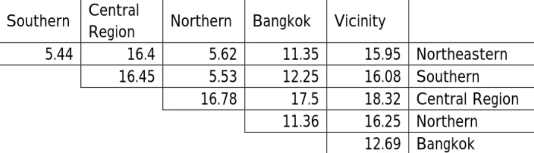
First, the degree of differentiation among the six regions is determined using the Krugman Index (Table 1). The southern, northern, and northeastern regions are found to be relatively similar, while the remaining three regions are relatively different from other regions. In these remaining regions, central region is different from Bangkok and its vicinity.
Second, the Theil index was calculated. The L-index was 0.270037. In the L-index, the share of intra inequality was about 70%, and the share of inter inequality was about 30%. This means that the difference between the two subregions in Thailand is smaller than the difference within the two subregions.
In Table 2, the Theil index for the 63 industries shows the industries differ between and within the two subregions of Thailand with regard to spread. The spread of industry between (1) Bangkok and its vicinities and (2) outside that of (1) is similar for the following: manufacture of footwear/ manufacture of knitted and crocheted fabrics and articles/ treatment and coating of metals; general mechanical engineering on a fee or contract basis/ manufacture of basic chemicals, except fertilizers nitrogen compounds/ manufacture of macaroni, noodles, couscous and similar farinaceous products/ manufacture of structural metal products/ processing and preserving of fish and fish product/ manufacture of bakery products/ manufacture of made-up, textile articles, except apparel/ manufacture of dairy products/ production of meat and meat
products/ manufacture other food products n.e.c./ and distilling, rectifying and blending of spirits; and ethylalcohol production from fermented materials.
In these industries, the distribution is similar within the two regions in terms of the treatment and coating of metals, and general mechanical engineering on a fee or contract basis/ manufacture other food products n.e.c., whereas the distribution is relatively different within the two regions in the processing and preserving of fish and fish products. The distribution is relatively similar within the two regions in the manufacture of pesticides and other agro-chemicals, and is dissimilar in the manufacture of vegetable and animal oils and fats/ manufacture of tobacco products/ manufacture of other transport equipment n.e.c./ and manufacture of railway and tramway locomotives and rolling stock.
The industry which is dissimilar between the two regions is the manufacture of aircraft and spacecraft. These industries tend to be relatively dissimilar between and within the two regions, and thus they show a tendency to concentrate.
Third, the L-index used again but this time excluding the south, north, and northeast regions; thus, Bangkok and its vicinity served as one group and the central area served as the other group. We remove the three similar regions, and add the two remaining relatively similar regions. The derived L-index is 0.95893; the share of inter-difference is about 88.8% and the share of between-difference is about 11.2%. The difference between the two subregions is small (Table 3) because most industries related with food are similar in both areas.
On the other hand, the difference in the intra regions was large in the following industries: manufacture of other transport equipment n.e.c./ manufacture coke oven product/ manufacture of man-made fibres/ manufacture of glass and glass products/ manufacture of office, accounting and computing machinery/ manufacture of engines and turbines, except aircraft, vehicle and cycle engines/ manufacture of structural non-refractory clay/manufacture of electric morots, generators and transformers/ manufacture of prepared animal feeds/ manufacture of tanks, reservoirs and containers of metal/ manufacture of starches and starch products/ processing of fruit and vegetables/and manufacture of grain mill products. No clear difference was obtained for the manufacture of motor vehicles because of the rogh administrative divisions used.
5. Conclusion
usage of areal statistics and the property of measures for understanding the difference between regions or industries. Some measures, Krugman index, L-index, Theil index, and the index used in Combes (2000) can be used to understand the difference between two regions’ industry, the dissimilarity within and between regions or industrial groups, and the difference between the varieties of industrial bases. However, as shown by the vague results produced by the various indices when applied to Thai statistics, we need to be cautious in interpreting what these indices suggest. In the final report of this research project, we will use the more fine administrative divisions to understand the industrial distribution and the difference of such distribution among regions.
References
Allison, P. D. (1978). “Measures of Inequality”, American Sociological Review, 43 (6), 865-880.
Atkinson, A. B. (1970). “On the Measurement of Inequality”, Journal of Economic Theory, 2, 244-263.
Balassa, B. (1965). “Trade Liberalization and Revealed Comparative Advantage”, Manchester School, 33, 99-123.
Burt, J.E. and G. M. Barber (1996). Elementary Statistics for Geographers, The Guilford Press, New York and London.
Combes, P. P. (2000). “Economic Structure and Local Growth: France, 1984-1993”, Journal of Urban Economics, 47, 329-355.
Cowell, F. A (1980). “On the Structure of Additive Inequality Measures”, The Review of Economic Studies, 47(3), 521-531.
Cowell, F. A (2009) Measuring Inequality, Oxford University Press,
http://darp.lse.ac.uk/papersDB/Cowell_measuringinequality3.pdf .
Cowell, F. A and K. Kuga (1980). “Additivity and the Entropy Concept: An Axiomatic Approach to Inequality Measurement”, Journal of Economic Theory, 25, 131-143
Cutrini, E. (2009) “Using Entropy Measures to Disentangle Regional from National Localization Patterns”, Regional Science and Urban Economic, 39, 243-250. De Benedictis, L. and M. Tamberi (2001). “A note on the Balassa Index of Revealed
Comparative Advantage”, Working Papers from Universita' Politecnica delle Marche (I), Dipartimento di Economia, No 158.
Duncan, O. D., R. P. Cuzzort and B. Duncan (1960). Statistical Geography, The Free Press, Illinois.
Encaoua, D. and A. Jacquemin (1980). “Degree of Monopoly, Indices of Concentration and Threat of Entry”, International Economic Review, 21(1), 87-105.
Hall, B. H., A. Jaffe, and M. Trajtenberg (2001). “The NBER Patent Citations Data File: Lessons, Insights, and Methodological Tools” in Jaffe and Trajtenberg, Patents, Citations, and Innovations, Cambridge, MA: The MIT Press.
Hart, P. E. (1975) “Moment Distributions in Economics: An Exposition”, Journal of Royal Statistical Society. Series A (General), 138 (3), 423-434.
Henderson, V., A. Kuncoro and M. Turner (1995). “Industrial Development in Cities”, The Journal of Political Economy, 103(5), 1067-1090.
Herfindahl, O. C. (1959). Copper Costs and Prices: 1870-1957, Baltimore: The Johns Hopkins Press.
Hirschman, A. O. (1945) National Power and the Structure of Foreign Trade, Berkeley and Los Angeles: University of California Press,
Hoover, Jr. E. M. (1936) “The Measurement of Industrial Localization”, The Review of Economics and Statistics, 18 (4), 162-171.
Isard, W. (1960) Method of Regional Analysis: an Introduction to Regional Science, Cambridge, London: The M.I.T. Press.
Krieger-Boden, C., E., Morgenroth and G. Petrakos (2008). The Impact of European Integration on Regional Structural Change and Cohesion, UK: Routledge. Krugman, P. (1991). Geography and Trade, Cambridge, London: The M.I.T. Press. Lorenz, M.O. (1905). “Method of Measuring the Concentration of Wealth”,
Publications of the American Statistical Association, 9 (70), 209-219.
Maliza, E. E. and S. Ke (1993). “The Influence of Economic Diversity on Unemployment and Stability”, Journal of Regional Science, 33(2), 221-235.
Midelfart-Knarvik, K. H., H. G. Overman, S. J. Redding and A. J. Venables (2002). “Integration and Industrial Specialization in the European Union”, Revue Economique, 53(3): 469-481.
Rey, S. J. (2001). “Spatial Analysis of Regional Income Inequality”, Urban/Regional 0110002, EconWPA.
Shanon, C. E. (1948). “The Mathematical Theory of Communication”, The Bell System Technical Journal, 27: 379–423 and 623–656.
Shorrocks, A. F. (1988) “Aggregation Issues in Inequality Measures” in W. Eichhorn (Ed.). Measurement in Economics: Theory and Applications of Economic Indices,. Heidelberg, Physica-Verlag HD.
Theil, H. (1967). Economics and Information Theory, Amsterdam: North-Holland Publishing Company.
Table 1: Degree of difference between six regions: Krugman index.
Southern Central
Region Northern Bangkok Vicinity
5.44 16.4 5.62 11.35 15.95 Northeastern 16.45 5.53 12.25 16.08 Southern
16.78 17.5 18.32 Central Region 11.36 16.25 Northern
12.69 Bangkok
Source: calculated by author. Note: Numbers are rounded.
Table 2: Theil index for 63 industries and six regions in Thailand
Category of industry Theil index within regions Theil index between regions
Manufacture of footwear 0.2238 0
Manufacture of knitted and crocheted fabrics and articles 0.3231 0
Treatment and coating of metals; general mechanical engineering on a fee or contract basis 0.0304 0.0001
Manufacture of basic chemicals, except fertilizers nitrogen compounds 0.2669 0.002
Manufacture of macaroni, noodles, couscous and similar farinaceous products 0.1899 0.0021
Manufacture of structural metal products 0.1685 0.007
Processing and preserving of fish and fish product 0.7055 0.0072
Manufacture of bakery products 0.0801 0.0077
Manufacture of made-up, textile articles, except apparel 0.2327 0.0084
Manufacture of dairy products 0.0214 0.0087
Production of meat and meat products 0.1384 0.0088
Manufacture other food products n.e.c. 0.0292 0.0098
Distilling, rectifying and blending of spirits; ethylalchol production from fermented materials 0.0316 0.0098
Manufacture of motor vehicle 0.2934 0.0151
Manufacture of vegetable and animal oils and fats 0.7414 0.0152
Manufacture of jewellery and related articles 0.2129 0.0201
Manufacture of electronic valves and tubes and other electronic components 0.3874 0.0207
Manufacture of bodies(coachwork) for motor vehicles; manufacture of trailers and semi-trailers 0.0414 0.0245
Manufacture of wearing apparel, except fur apparel 0.1456 0.0262
Manufacture of non-structural non-refractory ceramic ware 0.2394 0.0271
Manufacture of medical and surgical equipment and or orthopaedic appliances 0.106 0.0281
Manufacture of musical instrument 0.2419 0.0409
Manufacture of furniture 0.1832 0.042
Manufacture of tabaco products 1.0622 0.0532
Preparation and spining of textile fibres; weaving of textiles 0.0611 0.0559
Manufacture of tanks, reservoirs and containers of metal 0.3909 0.062
Manufacture of motorcycles 0.0658 0.0683
Manufacture of pulp, paper and paper board 0.0693 0.0692
Manufacture of rubber tyres and tubes; retreading and rebuilding of rubber tyres 0.5955 0.0695
Manufacture of other general purpose machinery 0.0411 0.0739
Manufacture of optical instruments and photographic equipment 0.3866 0.087
Building and repairing ships 0.2915 0.1053
Manufacture of articles of concrete, cement and plaster 0.0302 0.1071
Forging, pressing ,stamping nad roll-forming of metal; powder metallurgy 0.0215 0.1088
Manufacture of prepared animal feeds 0.2712 0.1124
Manufacture of basic iron and steel 0.1156 0.1152
Manufacture of electric morots, generators and transformers 0.4839 0.1354
Manufacture of sugar 0.0715 0.1368
Processing of fruit and vegetables 0.1528 0.1468
Manufacture of refined petroleum products 0.5251 0.1781
Manufacture of office, accounting and computing machinery 0.6998 0.1809
Dressing and dyeing of fur; manufacture of articles of fur 0.1048 0.1874
Tanning and dressing of leather 0.0424 0.1875
Manufacture coke oven product 0.6799 0.1982
Manufacture of glass and glass products 0.5927 0.1986
Printing 0.2847 0.2081
Manufacture of starches and starch products 0.3688 0.2495
Sawmilling and planing of wood 0.1337 0.2509
Manufacture of man-made fibres 0.6738 0.2564
Manufacture of bicycles and invalid carriages 0.2443 0.2613
Manufacture of soft drinks; bottling of mineral waters 0.3569 0.2736
Manufacture of pesticides and other agro-chemical 0.0089 0.3031
Manufacture of structural non-refractory clay 0.1197 0.3323
Manufacture of plastic products 0.018 0.3492
Publishing of books, brochures, musical books and other publications 0.4182 0.3587
Finishing of textiles 0.2072 0.3699
Recycling of metal waste and scrap 0.0731 0.4124
Manufacture of grain mill products 0.603 0.5011
Manufacture of other transport equipment n.e.c. 0.7623 0.6272
Manufacture of railway and tramway locomotives and rolling stock 1.7591 0.6431
Manufacture of aircraft and spacecraft 0.5875 0.7458
Table 3: Theil Index for 63 industries and three regions in Thailand
Category of industry Theil index within regions Theil index between regions
Manufacture of knitted and crocheted fabrics and articles 0.5062 0
Manufacture of footwear 1.1662 0
Treatment and coating of metals; general mechanical engineering on a fee or contract basis 0.8759 0.0001
Manufacture of basic chemicals, except fertilizers nitrogen compounds 1.1267 0.002
Manufacture of macaroni, noodles, couscous and similar farinaceous products 0.7663 0.0021
Manufacture of structural non-refractory clay 0.1769 0.007
Processing and preserving of fish and fish product 0.601 0.0072
Manufacture of bakery products 0.7737 0.0077
Manufacture of made-up, textile articles, except apparel 0.4839 0.0084
Manufacture of dairy products 0.6851 0.0087
Production of meat and meat products 1.2079 0.0088
Distilling, rectifying and blending of spirits; ethylalchol production from fermented materials 0.5948 0.0098
Manufacture other food products n.e.c. 0.8607 0.0098
Manufacture of motor vehicle 1.0256 0.0151
Manufacture of vegetable and animal oils and fats 0.5197 0.0152
Manufacture of jewellery and related articles 0.9225 0.0201
Manufacture of electronic valves and tubes and other electronic components 0.0065 0.0207
Manufacture of bodies(coachwork) for motor vehicles; manufacture of trailers and semi-trailers 0.6763 0.0245
Manufacture of wearing apparel, except fur apparel 0.4104 0.0262
Manufacture of non-structural non-refractory ceramic ware 0.7649 0.0271
Manufacture of medical and surgical equipment and or orthopaedic appliances 0.4882 0.0281
Manufacture of musical instrument 0.0192 0.0409
Manufacture of furniture 0.1296 0.042
Manufacture of tabaco products 0.8286 0.0532
Preparation and spining of textile fibres; weaving of textiles 0.3937 0.0559
Manufacture of tanks, reservoirs and containers of metal 1.5816 0.062
Manufacture of motorcycles 0.5527 0.0683
Manufacture of pulp, paper and paper board 0.6015 0.0692
Manufacture of rubber tyres and tubes; retreading and rebuilding of rubber tyres 1.2575 0.0695
Manufacture of other general purpose machinery 0.599 0.0739
Manufacture of optical instruments and photographic equipment 0.3977 0.087
Building and repairing ships 0.7632 0.1053
Manufacture of articles of concrete, cement and plaster 1.2177 0.1071
Forging, pressing ,stamping nad roll-forming of metal; powder metallurgy 0.4735 0.1088
Manufacture of prepared animal feeds 1.6948 0.1124
Manufacture of basic iron and steel 0.6071 0.1152
Manufacture of electric morots, generators and transformers 1.7798 0.1354
Manufacture of sugar 1.3302 0.1368
Processing of fruit and vegetables 1.5715 0.1468
Manufacture of refined petroleum products 1.8585 0.1781
Manufacture of office, accounting and computing machinery 1.9802 0.1809
Dressing and dyeing of fur; manufacture of articles of fur 0.4796 0.1874
Tanning and dressing of leather 0.3641 0.1875
Manufacture coke oven product 1.9918 0.1982
Manufacture of glass and glass products 1.9061 0.1986
Printing 0.4983 0.2081
Manufacture of starches and starch products 1.5967 0.2495
Sawmilling and planing of wood 1.3017 0.2509
Manufacture of man-made fibres 2.0117 0.2564
Manufacture of bicycles and invalid carriages 0.5377 0.2613
Manufacture of soft drinks; bottling of mineral waters 0.5111 0.2736
Manufacture of pesticides and other agro-chemical 0.2308 0.3031
Manufacture of structural non-refractory clay 1.9874 0.3323
Manufacture of plastic products 0.1095 0.3492
Publishing of books, brochures, musical books and other publications 0.622 0.3587
Finishing of textiles 0.3284 0.3699
Recycling of metal waste and scrap 0.001 0.4124
Manufacture of grain mill products 1.5631 0.5011
Manufacture of other transport equipment n.e.c. 2.2974 0.6272
Manufacture of railway and tramway locomotives and rolling stock 0 0.6431
Manufacture of aircraft and spacecraft 0.5875 0.7458