A discussion of nonnegative solutions of elliptic equations on symmetric domains (Nonlinear Partial Differential Equations, Dynamical Systems and Their Applications)

A

discussion

of

nonnegative

solutions

of

elliptic

equations

on

symmetric

domains*

P. Pol\’a\v{c}ik\dagger

School of Mathematics, University ofMinnesota

Minneapolis, MN 55455

Abstract. In this note we summarize our recent results on

nonnega-tive solutions of nonlinearelliptic equations onreflectionallysymmetric

domains. We discuss symmetry properties ofsuchsolutions, the

struc-ture oftheir noda$I$ set, and the existence and multiplicity of solutions

with a nontrivial nodal set.

Contents

1 Introduction 2

2 Notation and hypotheses 4

3 Symmetry properties of nonnegative solutions 6

4 Existence and nonexistence results 7

4.1 Examples 8

4.2 Nonexistence of nonnegative solutions with a nontrivial nodal

set 10

5 Uniqueness and multiplicity results 12

*Prepared for the Proceedings of the International Conference on Partial Differential Equations-in honor of Hiroshi Matano

1

_Introduction

Consider a nonlinear elliptic problem ofthe form

$F(x, u, Du, D^{2}u)=0, x\in\Omega$_{, (1.1)}

$u=0, x\in\partial\Omega$. (1.2)

Here $\Omega$ is a bounded domain in $\mathbb{R}^{N}$

, which is reflectionally symmetric about

the hyperplane

$H_{0}=\{x=(x_{1}, x’)\in \mathbb{R}\cross \mathbb{R}^{N-1}:x_{1}=0\}$

andconvexin thedirection$e_{1}$ $:=(1,0, \ldots, 0)$

.

The nonlinearity $F$is assumed

to be sufficiently regular, elliptic, and symmetric, so that in particular the

equation is invariant under the reflection in $H_{0}$ (see Section 2 for the precise

hypotheses). For example, the semilinear problem

$\triangle u+f(x’, u)=0, x=(x_{1}, x’)\in\Omega$, (1.3)

$u=0, x\in\partial\Omega$, (1.4)

where $f$ : $\mathbb{R}^{N-1}\cross \mathbb{R}arrow \mathbb{R}$is continuous in all variables and Lipschitz in

$u$, is

admissible for our results without any additional assumption on $f.$

By a celebrated theorem of Gidas, Ni, and Nirenberg [13], and its

gener-alization to nonsmooth domains given by Berestycki and Nirenberg [3] (see

also Dancer’s result in [8]$)$, each positive (classical) solution _$u$ of (1.1), (1.2) is even in $x_{1}$:

$u(-x_{1}, x’)=u(x_{1}, x’) ((x_{1}, x’)\in\Omega)$, (1.5)

and decreasing with increasing $|x_{1}|$:

$u_{x_{1}}(x_{1}, x’)<0 ((x_{1}, x’)\in\Omega, x_{1}>0)$. (1.6)

This result was proved using the method of moving hyperplanes introduced

by Alexandrov [1] and further developed and applied in a symmetry

prob-lem by Serrin [25]. We refer the reader to the surveys [2, 16, 17, 18], the

monographs [9, 12, 24], or the more recent paper [6], for perspectiveson this

theorem, related results, and many other references.

The above symmetry and monotonicity theorem is not valid in general

ifthe solution $u$ is assumed to be nonnegative, rather than strictly positive:

consider, for example, the function $u(x)=1+\cos x$ _{as a solution of} $u”+$

$u-1=0$

on

$\Omega=(-3\pi, 3\pi)$

.

Note, however, that in this example $u$ still has

about the center of the

interval

between any two successive

zeros.

It is not

hard to prove that a similar symmetry result is valid for the nonnegative

solutions of any problem (1.3), (1.4) in

one

space dimension (in the

one-dimensional case, $\Omega=(-\ell, \ell)$ for

some

$\ell>0$, and there is

no

variable $x’$).

It is natural to ask whether in higher dimension, nonnegative solutions

also have some symmetry properties. One would also like to know how the

nodal set of such solutions

can

look like and whether it has

some

symmetry

itself. We address these problems in Section 3. The theorem

we

give there

states, roughly speaking, that each nonnegativesolutions$u$of (1.1), (1.2) has

a similar symmetry structure

as

solutions in one dimension: it is symmetric

about $H_{0}$ and, if $u\not\equiv 0$ and $u$ is not strictly positive in $\Omega$, the nodal set

of $u$ divides $\Omega$ into a finite number of reflectionally symmetric subdomains

(nodal domains) inwhich $u$ has the usual Gidas-Ni-Nirenberg symmetry and

monotonicity properties.

Discussing nonnegative solutions with a nontrivial nodal set,

we

have

an

obligation to address the problem of existence of such solutions. Using the

one-dimensional example mentioned above, it is not difficult to find such

solutions for

some

problems

on a

rectangle. However, it is not at all

a

trivial

matter to determine whether such solutions

can

be found

on

other domains

and whether they

can

be found for

more

specffic problems, like the spatially

homogeneous semilinear equations. These issues are discussed in Section 4,

where we summarize known examples of solutions with a nontrivial nodal

set and mention several results on the nonexistence of such solutions under

various additional conditions

on

the nonlinearity and/or the domain.

Our next

concern

is the multiplicity of nonnegative solutions with a

nontrivial nodal set, in case such solutions do exist. For one-dimensional

problems (1.3), (1.4), a phase-plane analysis reveals that if a solution has

interior zeros, then it’s derivative has to vanish at the boundary points,

that is, such

a

solution satisfies simultaneously the Dirichlet and Neumann

boundary conditions. The uniqueness for the Cauchy problem for the

sec-ond order $ODE$ therefore implies that the solution is uniquely determined.

Surprisingly perhaps, a similar uniqueness result holds for a large class of

domains, not necessarily smooth, in any dimension. For general domains,

the number of solutions with interior zeros is finite. See Section 5, for a

2

Notation

and

hypotheses

In this section we state the hypotheses used throughout the paper. First

recall that the standing hypothesis on $\Omega\subset \mathbb{R}^{N}$ is that

it is a bounded

domain, which is $x_{1}$

-convex

$(or$ convex $in the$ direction _{$e_{1}=(1,0, \ldots, 0)$})

and symmetric about the hyperplane $H_{0}=\{(x_{1}, x’)\in \mathbb{R}^{N} : x_{1}=0\}.$

To formulate our hypotheses on the nonlinearity $F$, let $S$ denote the

space of$N\cross N$ symmetric (real) matrices and $\mathcal{B}$ $:=\mathbb{R}\cross \mathbb{R}^{N}\cross S$

.

Let _$Q$ be

the transformation on $\mathcal{B}$ defined

by

$Q(u,p, q)=(u, -p_{1},p_{2}, \ldots,p_{N},\overline{q})$, (2.1)

$\overline{q}_{ij}=\{\begin{array}{ll}-q_{ij} if exactly one of i, j equals 1,q_{ij} otherwise.\end{array}$

We

assume

that $F$ : _{$(x, u,p, q)\mapsto F(x, u,p, q)$} : $\overline{\Omega}\cross \mathcal{B}arrow \mathbb{R}$, satisfies the

following conditions.

(Fl) (Regularity) $F$ is continuous on $\overline{\Omega}\cross \mathcal{B}$

and Lipschitz in $(u,p, q)$: there

is $\beta_{0}>0$ such that

$|F(x, u,p, q)-F(x,\tilde{u},\tilde{p},\tilde{q})|\leq\beta_{0}|(u,p, q)-(\tilde{u},\tilde{p},\tilde{q})|$

$((x, u,p, q), (x,\tilde{u},\tilde{p},\tilde{q})\in\overline{\Omega}\cross \mathcal{B})$

.

(2.2)

Moreover, $F$ is differentiable with respect to

$q$ on $\Omega\cross \mathcal{B}$ and its

deriva-tives $F_{q_{ij}},$ $i,j=1,$

$\ldots,$$N$, are Lipschitz (in all variables) on $\Omega\cross \mathcal{B}.$

(F2) _{(Ellipticity) There is a constant} $\alpha_{0}>0$ such that

$F_{q_{ij}}(x, u,p, q)\xi_{i}\xi_{j}\geq\alpha_{0}|\xi|^{2} ((x, u,p, q)\in\Omega\cross \mathcal{B}, \xi\in \mathbb{R}^{N})$

.

(2.3)

Here and below we use the summation convention (summation over

repeated indices). For example, in the above formula the left hand

side represents the sum over $i,j=1,$ $\ldots,$ $N.$

(F3) (Symmetry) $F$ is independent of

$x_{1}$ and for any $(x, u,p, q)\in\Omega\cross \mathcal{B}$

one has

$F(x, Q(u,p, q))=F(x, u,p, q) (=F((0, x’), u,p, q))$

.

We consider classical solutions $u$ of (1.1), (1.2). By this

we mean

func-tions $u\in C^{2}(\Omega)\cap C(\overline{\Omega})$ such that (1.1), (1.2) are satisfied everywhere.

When _{considering fully nonlinear equations, we shall require the}

(U) For $i,j=1,$ $\ldots,$$N$, the derivatives $u_{x_{i}x_{j}}$

are

locally Lipschitz

continu-ous on

$\Omega.$

We remark that one can often establish the validity of (U) for each

classical solution if additional assumptions are made on $F.$ $A$ sufficient

condition is that $F$ is differentiable (in all variables) on $\Omega\cross \mathcal{B}$ and all its

first order derivatives

are

locally H\"older continuous (see [14, Lemma 17.16]).

The main

reason

for thecondition (U) isthat

some

theoremsstatedbelow

depend on the unique continuation and related results for linear equations

related to (1.1), such

as

the linear equation for the difference of two solutions

of (1.1). For the unique continuation to apply, the leading coefficients in the

linear equation must be (locally) Lipschitz continuous. This is guaranteed

by the Lipschitz continuity of the derivatives $F_{q_{ij}}$, as assumed in (Fl), and

condition (U). For morespecific equations, condition (Fl) alone is sufficient.

This is the case, for example, if (1.1) is quasilinear, that is,

$F(x, u,p, q)=A_{ij}(x, u,p)q_{ij}+f(x, u,p)$ $((x, u,p)\in(\overline{\Omega}\cross \mathcal{B}))$ (2.4)

for

some

functions $A_{ij}$ and $f$

.

Note that in this case, the last requirement

in (Fl) translates to the Lipschitz continuity of the functions $A_{ij},$ $i,j=$

$1,$

$\ldots,$$N$, in

$(x, u,p)\in\Omega\cross \mathbb{R}^{N+1}$

Condition (Fl) implies that $F$ differentiable with respect to $u,$ $p,$ $q$

al-most everywhere. In Section 5,

we

shall need the stronger differentiability

property:

(Fla) $F$ is everywhere differentiable with respect to $u,$ $p,$ $q.$

The

reason

for this condition is

an

application of the chain rule, which does

not always hold for Lipschitz functions. However, for semilinear equations

(1.3), condition (Fla) is not needed (see the remark at the end of Section

5$)$

.

The following notation is used throughout the paper (here $\lambda\in \mathbb{R}$ and

$U\subset\Omega)$:

$H_{\lambda}:=\{x\in \mathbb{R}^{N}:x_{1}=\lambda\},$

$\Gamma_{\lambda}:=H_{\lambda}\cap\Omega,$

$\ell$ _{$:= \sup\{x_{1}\in \mathbb{R}$} : $(x_{1}, x’)\in\Omega$ for some $x’\in \mathbb{R}^{N-1}\}.$

$\Sigma_{\lambda}^{U}:=\{x\in U:x_{1}>\lambda\}.$

When $U=\Omega$, we omit the superscript $U=\Omega$, thus

Let $P_{\lambda}$ stand for the reflection in the hyperplane $H_{\lambda}$

.

Note that since $\Omega$ is

convex in $x_{1}$ and symmetric in the hyperplane $H_{0},$ $P_{\lambda}(\Sigma_{\lambda})\subset\Omega$ for each

$\lambda\in[0, \ell)$ and $\Sigma_{0}$ is connected $(for \lambda>0, \Sigma_{\lambda} may not be$ connected)

.

For any function $z$

on

$\overline{\Omega}$

, we define $V_{\lambda}z$ by

$V_{\lambda}z(x)=z(P_{\lambda}x)-z(x) (x\in\overline{\Sigma}_{\lambda})$. (2.5)

3

Symmetry properties

of

nonnegative

solutions

The following theorem describes the symmetry structure of nonnegative

so-lutions of (1.1), (1.2).

Theorem 3.1 ([20]). Assume that $(F1)-(F3)$ _{hold and let}$u$ be

a

nonnegative

solution

_of

(1.1), (1.2). Further assume that (U) holds or $F$ is

of

the

form

(2.4). Then either $u\equiv 0$ $($hence, necessarily, $F(\cdot, 0,0,0)\equiv 0$) or else there

exist $m\in \mathbb{N}$ and constants $\lambda_{1},$

$\ldots,$$\lambda_{m}$ with the following properties:

(i) $0=\lambda_{m}<\lambda_{m-1}<\cdots<\lambda_{1}<\ell.$

(ii) For $i=1,$ $\ldots,$$m,$ $V_{\lambda_{i}}u\equiv 0$ on a connected component

of

$\Sigma_{\lambda_{i}}$

.

In

particular, $a\mathcal{S}\Sigma_{0}$ is connected, $V_{0}u\equiv 0$ in $\Sigma_{0}$, that is, _$u$ is even in

$x_{1}.$

(iii) There are mutually disjoint open $set_{\mathcal{S}}G_{i}\subset\Omega,$ $i=1,$

$\ldots,$$m$, with $G_{m}$

$po\mathcal{S}$sibly empty, such that the following $\mathcal{S}tatement\mathcal{S}$ are true;

$(a)\emptyset\neq G_{i}\subset\Sigma_{0} (i=1, \ldots, m-1)$

.

$(b) \overline{\Omega}=\overline{G}_{m}\cup\bigcup_{i=1}^{m-1}(\overline{G}_{i}\cup P_{0}(\overline{G}_{i}))$.

$(c)$ For $i=1,$

$\ldots,$ $m$, the set

$G_{i}$ is _{$x_{1}$}-convex and _{$P_{\lambda_{i}}(G_{i})=G_{i}.$}

$(d)$ $Fori=1,$

$\ldots,$$m$, one $ha\mathcal{S}u>0$ in $G_{i},$ $u=0on\partial G_{i},$ $V_{\lambda_{i}}u\equiv 0$

in $Gb$, and $u_{x_{1}}<0$ in $\Sigma_{\lambda_{i}}^{G_{i}}$

If $m=1$ $($and _{$\lambda_{1}=0)$}, statements (ii) and (iii) give the usual symmetry

and monotonicity properties of a positive solution $u$

.

In the general case,

(ii), (iii) show that the nodal set of$u,$ $u^{-1}(0)$, divides $\Omega$ into a finite number

of open reflectionally symmetric subsets $G_{m},$ $G_{i},$ $P_{0}(G_{i}),$ $i=1,$

$\ldots,$ $m-1$, in

each ofwhich $u$ is positive, and has the usual Gidas-Ni-Nirenberg symmetry

and monotonicity properties. In is also proved in [20] that each of thesets $G_{i}$

has finitely many connected components. We remark that, although in [20]

the formulation of condition (U) is stronger in that the Lipschitz continuity

of the functions $u_{x_{i}x_{j}}$ on

$\Omega$ is required, just the local Lipschitz continuity is

A related symmetry result for nonnegative solutions ofvariational

prob-lems is proved in [4]. It says that for each subdomain $U$ of $\Omega$ in which $u>0$

and $u_{x_{1}}>0$, the graph of $u$ contains a part reflectionally symmetric to

$\{(x, u(x)) : x\in U\}$

.

The basic method of [4] is the continuous Steiner

sym-metrization. In [20],

a

modification of the method of moving hyperplanes

is used. The latter applies to more general equations, but requires stronger

regularity assumptions.

4

Existence

and

nonexistence

results

As we will see shortly, there

are

domains $\Omega$ and nonlinearities $f=f(x’,u)$,

such that the semilinear problem (1.3), (1.4) admits a solution with a

non-trivial nodal set in $\Omega$ (here “nontrivial”

means

different from $\Omega$ and $\emptyset$). On

the other hand, there

are

domains

on

which there

are no

such solutions,

no

matter how the nonlinearity is chosen. An example is any $C^{1}$

convex

domain

in $\mathbb{R}^{2}$ whose boundary contains a line segment parallel to the _{$x_{2}$} axis. This

was shown in [20, Proposition 2.7] for semilinear problems (1.3), (1.4). By

similar arguments, one can prove that on such a domain there

can

be no

solutions with a nontrivial nodal set for any fully nonlinear problem (1.1),

(1.2) (assuming that conditions (Fl)$-(F3)$, (Fla), and (U) are in effect). We

refer the reader to [20] for some explanations as to why the existence of

solutions with a nontrivial nodal set imposes restriction on the domain and

how this is related to

some

results concerning overdetermined problems.

We do not have

a

good understanding of domains which support

so-lutions with a nontrivial nodal set, let alone any general classffication of

such domains. $A$ classification problem of this sort can be formulated in

the context of general fully nonlinear problems (1.1), (1.2) or more specific

problems, such

as

(1.3), (1.4). We cannot say much about either.

How-ever,

we

do have

some

general nonexistence results concerning the spatially

homogeneous problem

$\Delta u+f(u)=0, x\in\Omega$, (4.1)

$u=0, x\in\partial\Omega$, (4.2)

see Section 4.2 below. In Section 4.1, we summarize known examples of

semilinear problems (1.3), (1.4) admitting solutions with a nontrivial nodal

set. As of today, there seem to be no known examples of such solutions for

the homogeneous multidimensional problem (4.1), (4.2). Results in Section

4.2 completely rule out such examples with smooth domains,

or

in the case

4.1

Examples

In all examples given in this section, $\Omega$ is a planar domain, hence we

use

the

simplified notation $(x, y)=(x_{1}, x’)$

.

We consider problems of the form

$\triangle u+\mu u+h(y)=0, (x, y)\in\Omega$, (4.3)

$u=0, (x, y)\in\partial\Omega$, (4.4)

where $\Omega\subset \mathbb{R}^{2}$

satisfies the standing hypothesis, $\mu$ is a positive constant, and

$h$ a continuous function of

$y$ only. Thus this is a problem of the form (1.3),

(1.4). For suitable $\Omega,$

$\mu$, and $h$, as specified below, there is a nonnegative

solution $u$ with interior nodal curves. In Figures 1-4, the solid lines indicate

the nodalcurves ofthe solution$u$ and thedashed lines indicate the symmetry

hyperplanes (lines) for the nodal domains of $u$ (cp. Theorem 3.1).

We start with two explicit examples.

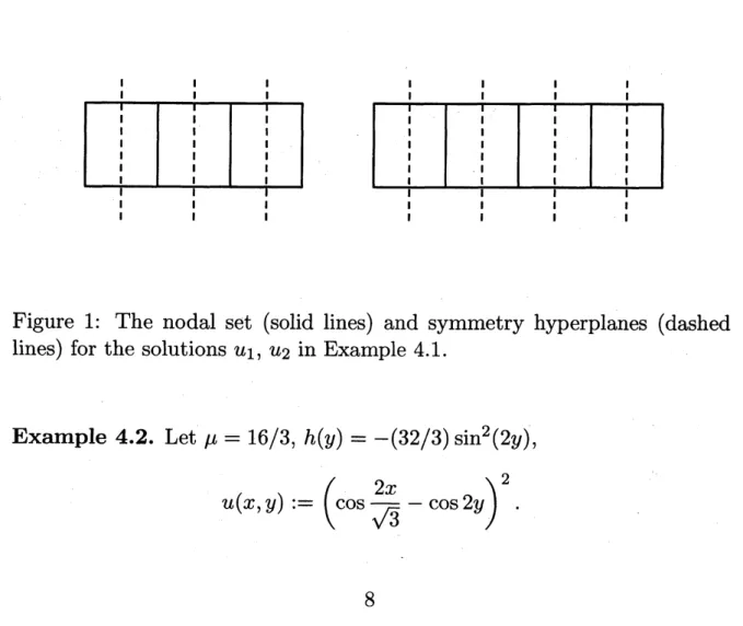
Example 4.1. Let $\mu=2,$ $h(y)=-\sin y,$ $u_{1}(x, y)$ $:=(1+\cos x)\sin y$, and

$u_{2}(x, y)$ $:=(1-\cos x)\sin y$

.

Then, for any $k\in \mathbb{N}$, the functions_{$u_{1}$} and _{$u_{2}$} are

nonnegative solutions of (4.3), (4.4) on $\Omega=(-(2k+1)\pi, (2k+1)\pi)\cross(0, \pi)$

and $\Omega=(-2k\pi, 2k\pi)\cross(0, \pi)$, respectively.

1 1 1 1 1 1 1 $1$ 1 1 1 1 1 1 I I I I 1 I I I I I I I I I I I I I

Figure 1: The nodal set (solid lines) and symmetry hyperplanes (dashed

lines) for the solutions $u_{1},$ $u_{2}$ in Example 4.1.

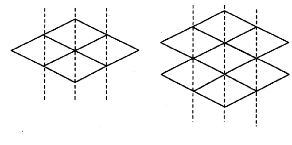
Example 4.2. Let $\mu=16/3,$ $h(y)=-(32/3)\sin^{2}(2y)$_,

The nodal lines of $u$

are

given by $y=\pm x/\sqrt{3}+k\pi,$ $k\in \mathbb{Z}$,

and the

func-tion $u$ is a nonnegative solution of (4.3), (4.4)

on

any symmetric domain

whose boundary consists of segments from these lines. Figure 2 shows two

possibilities.

111

1 1

111

1!

Figure 2: The nodal set and symmetry lines for solutions in Example 4.2.

In the previous two examples, the interior nodal set of $u$ consists of line

segments. This is different in the next example, where the nodal set consists

of non-flat analytic

curves.

Example 4.3. The domain $\Omega$ and the nodal

curves

of

$u$

are

as

in Figure 3.

The definition of $\Omega,$

$\mu$, and $h$ is not so simple and explicit here;

we

refer the

reader to [20, Section 5] for the detailed construction.

Figure 3: The domain and nonflat nodal lines of a solution.

The domains in the previous examples have corners. The next theorem

shows that even on smooth domains one can find solutions with a nontrivial

Theorem 4.4 ([23]). There exist a constant $\mu>0$, a continuous

function

$h:\mathbb{R}arrow \mathbb{R}$, and a bounded analytic domain $\Omega\subset \mathbb{R}^{2}$ satisfying the standing

hypothesis such thatproblem (4.3), (4.4) has a nonnegative solution $u$ whose

nodal set in $\Omega$ consists

of

two analytic curves (see Figure 4).

Figure 4: The domain $\Omega$, and the nodal set and symmetry lines of the solution

$u$

from Theorem 4.4.

A few words about how the above examples have been found. The

constructions link the solutions of (4.3) to eigenfunction of the Laplacian.

Specifically, if $u$ is

a

solution of (4.3), then _{$v=u_{x}$} satisfies $\triangle v+\mu v=0$ in

$\Omega$

.

Moreover, if _{$u\geq 0$} in $\Omega$, then $v=0$ on all nodal

curves

of

$u$ in $\Omega$

.

Also,

one has $v=0$ on $H_{0}$ and all the other symmetry lines of $u$ parallel to $H_{0}.$

Thus a key prerequisite for our construction is an eigenvalue-eigenfunction

pair $(\mu, v)$ of the Laplacian, such that $v$ has a suitable nodal structure.

The solution $u$ of (4.3), $(4\backslash 4)$, for some function $h$, is then found as an

antiderivative of $v$ with respect to _$x.$

4.2

Nonexistence of nonnegative solutions

with

a

nontrivial

nodal

set

Some resultsonthenonexistence of solutions with anontrivialnodalset have

been available for a long time, in particular for the homogeneous problem

(4.1), (4.2). In [5], such a result is proved if $\Omega$ is a ball in $\mathbb{R}^{N}(N\geq 2)$

(see also the monographs [9, 12] for the proofand a discussion ofthis result;

an extension to quasilinear radial problems can be found in [24]$)$

.

More

generally, nonexistence results for (4.1), (4.2)

can

be found in [15] or [7],

where $\Omega$ is a $C^{2}$ domain satisfying, in addition to the standing hypothesis,

a geometric condition: a sort of strict $x_{1}$-convexity in [15] and convexity

the strict positivity of nonnegative

nonzero

solutions

was

given in [10]. It

requires, roughly speaking, that for any $\delta>0$ there be

a

two-dimensional

wedge $W$, such that if the tip of $W$ is translated to any point of $\partial\Omega$ with

$x_{1}\geq\delta$, then $W$ is contained in $\overline{\Omega}$

.

Note that a rectangle, or a rectangle with

smoothed out corners, does not satisfy the geometric condition of [10]. The

results of [10] apply to equations (1.3) (and to a class of of fully nonlinear

equations), if they satisfy additional symmetry assumptions.

We

now

give two rather general nonexistence results for (4.1), (4.2). In

the first one, we deal with general smooth domains in $\mathbb{R}^{N},$ $N\geq 2.$

Theorem 4.5 ([19]). Let $\Omega$ be a $C^{2}$ bounded domain in $\mathbb{R}^{N},$ $N\geq 2$,

sat-isfying the standing hypothesis.

_If

$u\in C^{2}(\overline{\Omega})$ is a nonnegative solution

of

(4.1), (4.2)

_for

some

locally Lipschitz

_function

$f$ : $\mathbb{R}arrow \mathbb{R}$, then either $u\equiv 0$

or else $u>0$, hence $u$ has the symmetry and monotonicity properties (1.5)

and (1.6).

We remark that, by the Schauder theory, any classical solution of (1.1),

(1.2) belongs to $C^{2}(\overline{\Omega})$ (even to $C^{2+\alpha}(\overline{\Omega})$) if $\Omega$ is

a

$C^{2+\alpha}$ domain for

some

$\alpha\in(0,1)$

.

The next theorem gives the nonexistence for a large class of planar

do-malns.

Theorem 4.6 ([21]). Assume that $\Omega$ is a bounded domain in $\mathbb{R}^{2}$ satisfying

the standing hypothesis such that one

_of

the following conditions is

_satisfied:

(i) $\Omega$ is convex (not necessarily symmetric) in the direction $e_{2}=(0,1)$

(the direction

_of

the $x_{2}$ axis),

(ii) $\Omega$ is strictly

convex

in the direction

$e_{1},$

(iii) $\Omega$ is piecewise $C^{1,1}$

Let $f$ : $[0, \infty)arrow \mathbb{R}$ be a locally Lipschitz

function

such that

for

some

con-stants $\delta>0,$ $\alpha\in$ _{$(0,1] one has f|_{[0,\delta)}\in C^{1,\alpha}[0, \delta)$}.

If

$u\in C^{2}(\Omega)\cap C(\overline{\Omega})$ is

a nonnegative solution

_of

(1.1), (1.2), then either $u\equiv 0$ or else $u>0.$

Note that $\Omega$ is strictly convex in the direction

$e_{1}$ if

$\partial\Omega$ contains no

horizontal line segments $(that is,$ segments parallel $e_{1})$. Condition (iii) can

be weakened; we only need the boundary of $\Omega$ to be piecewise $C^{1,1}$

ne.ar

the

end points of the horizontal line segments contained in $\partial\Omega$

.

If there are no

5Uniqueness and multiplicity results

We mentioned in the introduction that in one-dimensional problems, the

uniqueness of the Cauchy problem implies the uniqueness of solutions with

a nontrivial nodal set. The

same can

be said of multidimensional problems

under some geometric conditions on $\Omega$, for example, if $\Omega$ is convex (in all

directions). This may be surprising at the first glance, as we are making no

smoothness assumptions on $\Omega$

.

To explain, recall that the symmetries of

$u$

(see Theorem 3.1) imply that a portion of $\partial\Omega$ is the reflection of a nodal

set of $u$

.

Now, the nodal set of $u$ is at the same time the nodal set of $u_{x_{1}}$

$(as u\geq 0)$, and the latter has some partial regularity properties, thanks to

well-known theorems for linear equations. One eventually shows that any

two solutions with a nontrivial nodal set in $\Omega$ vanish on a smooth portion of

$\partial\Omega$ together with their gradients. The uniqueness for the Cauchy problem

for elliptic equations then implies that any two such solutions coincide on

a

nonempty open subset. Consequently, by unique continuation, they coincide

everywhere in $\Omega$, which gives the uniqueness.

The above arguments give the uniqueness if $\Omega$ is convex or if other

geo-metric conditions are imposed. Without any additional conditions on $\Omega$, we

can prove that the number ofsolutions with a nontrivial nodal set is finite.

To give a precise statement, let $E_{nod}$ be the set of all nonnegative solutions

$u$ of (1.1), (1.2), which satisfy (U) and for which $u^{-1}(0)\cap\Omega\neq\emptyset.$

Theorem 5.1 ([22]). Assume that $(F1)-(F3)$, (Fla) hold. Then the set

$E_{nod}$ is

finite. If

the set $\Sigma^{\lambda}$

is connected

_for

each $\lambda>0$, then $E_{nod}$ has at

most one element.

Note that $\Sigma^{\lambda}$

is connected for each $\lambda>0$ if$\Omega$ is

convex

(in alldirections)

or, more generally, if it is convex in all directions perpendicular to $e_{1}.$

See [22] for the proof of

this

theorem and a more precise multiplicity

result giving an estimate on $|E_{nod}|$ in terms of $N=\dim\Omega$, the constants $\beta_{0},$

$\alpha_{0}$ from (Fl), (F2), and some geometric characteristics of $\Omega.$

The finite multiplicity result is of some importance in studies of the

parabolic problem associated with (1.1), (1.2). The solutions of (1.1), (1.2)

are equilibria for the parabolic problem, and the equilibria with \‘a nontrivial

nodal set play a distinguished role in the global dynamics (more details

on

this will appear in [11]$)$.

The multiplicity result have also some symmetry consequences for the

solutions of (1.1), (1.2) themselves. For example, if both $\Omega$ and _$F$ are

nontrivial nodal set must be symmetric withrespect

to

that

group

(otherwise

its group orbit yields infinitely many such solutions).

We conclude with a remark concerning assumption (Fla). The

argu-ments in [22] depend on the fact that the function $u_{x_{1}}$, which is of class

$C^{1,1}$

by (U), satisfies almost everywhere

a

linear equation with bounded

coeffi-cients. To

see

this just differentiate (1.1) with respect to $x_{1}$ using the chain

rule and the fact that $F$ is independent of $x_{1}$ (see condition (F3)). The

chain rule does not apply in general to Lipschitz functions, and this is the

only

reason

why we need condition (Fla). However,

one can use

different

arguments if the equation is semilinear,

as

in (1.3). Even without (Fla),

one can

show that $v=u_{x_{1}}$ is

a

solution of the equation

$\Delta v+a(x)v=0, x\in\Omega$, (5.1)

where $a(x)$ is a bounded measurable function. More specffically, $a(x)$ is

any bounded measurable which coincides with $f_{u}(x, u(x))$, except at the

points $x$ such that either $v(x)=u_{x_{1}}(x)=0$ (in which

case

the value of

$a(x)$ is irrelevant in (5.1)$)$ or _{$u_{x_{1}}\neq 0$} and the derivative $f_{u}$ does not exist at $(x’, u(x))$

.

It _{is not dfficult to show, using the Lipschitz continuity of}$f$with

respect to $u$, that the set of all points $x\in\Omega$ with the latter property has

measure zero.

One then proves that $u_{x_{1}}$ satisfies (5.1) almost everywhere by

considering the equation satisfied by $(u(x_{1}+\epsilon, x’)-u(x_{1}, x’))/\epsilon$ and taking

the limit

as

$\epsilon\searrow 0.$

References

[1] A. D. Alexandrov, A characteristic property

_of

spheres, Ann. Math.

Pura Appl. 58 (1962), 303-354.

[2] H. Berestycki, Qualitative properties

_of

positive solutions

_of

elliptic

equations, Partial differential equations (Praha, 1998), Chapman

&

Hall/CRC Res. Notes Math., vol. 406, Chapman

&

Hall/CRC, Boca

Raton, FL, 2000, pp. 34-44.

[3] H. Berestycki and L. Nirenberg, On the method

_of

moving planes and

the sliding method, Bol. Soc. Brasil. Mat. (N.S.) 22 (1991), 1-37.

[4] F. Brock, Continuous rearrangement and symmetry

_of

$\mathcal{S}$olutions

of

[5] A. Castro and R. Shivaji, Nonnegative solutions to a semilinear

Dirich-letproblem in a ball are positive and radially symmetric, Comm. Partial

Differential Equations 14 (1989), 1091-1100.

[6] F. Da Lio and B. Sirakov, Symmetry results

_for

viscosity solutions

_of

fully nonlinear uniformly elliptic equations, J. European Math. Soc. 9

(2007),

317-330.

[7] L. Damascelli, F. Pacella, and M. Ramaswamy, A $\mathcal{S}$trong maximum

principle

_for

a $clas\mathcal{S}$

of

non-positone singular elliptic problems, NoDEA

Nonlinear Differential Equations Appl. 10 (2003), no. 2, 187-196.

[8] E. N. Dancer, Some notes on the method

_of

moving planes, Bull.

Aus-tral. Math. Soc. 46 (1992), 425-434.

[9] Y. Du, Order structure and topological methods in nonlinear partial

differential

equations. Vol. 1, Series in Partial Differential Equations

and Applications, vol. 2, World Scientffic Publishing Co. Pte. Ltd.,

Hackensack, NJ, 2006.

[10] J. F\"oldes, On symmetry $propertie\mathcal{S}$

of

parabolic equations in bounded

domains, J. Differential Equations 250 (2011), 4236-4261.

[11] J. F\"oldes _{and P. Pol\’a\v{c}ik, (in preparation).}

[12] L. E. $\mathbb{R}$aenkel,

An introduction to maximum principles and

symme-try in elliptic problems, Cambridge Tracts in Mathematics, vol. 128,

Cambridge University Press, Cambridge, 2000.

[13] B. Gidas, W.-M. Ni, and L. Nirenberg, Symmetry and relatedproperties

via the maximum principle, Comm. Math. Phys. 68 (1979), 209-243.

[14] D. Gilbarg and N. S. Tirudinger, Ellipticpartial

_differential

equations

_of

$\mathcal{S}$econd order, Classics in Mathematics, Springer-Verlag, Berlin, 2001,

Reprint of the 1998 edition.

[15] P. Hess and P. Pol\’a\v{c}ik, Symmetry and convergence properties

_for

non-negative solutions

_of

nonautonomous $reaction-diffu\mathcal{S}ion$ problems, Proc.

Roy. Soc. Edinburgh Sect. A 124 (1994), 573-587.

[16] B. Kawohl, Symmetrization - or how to prove symmetry

of

solutions

to

a

PDE, Partial differential equations (Praha, 1998), Chapman

&

Hall/CRC _{Res. Notes} Math., vol. 406, Chapman

&

Hall/CRC, Boca

[17] W.-M. Ni, Qualitat ive properties

_of

solutions to elliptic problems,

Hand-book of Differential Equations: Stationary Partial Differential

Equa-tions, vol. 1 (M. Chipot and P. Quittner, eds.), Elsevier, 2004, pp.

157-233.

[18] P. Pol\’a\v{c}ik, Symmetry properties

_of

positive $\mathcal{S}$olutions

of

parabolic

equa-tions: a survey, Recent progress

on

reaction-diffusion systems and

vis-cositysolutions (W.-Y. Lin Y. Du, H. Ishii, ed.), World Scientffic, 2009,

pp. 170-208.

[19] –, Symmetry

of

nonnegative solutions

of

elliptic equations via a

result

_of

Serrin, Comm. Partial Differential Equations 36 (2011),

657-669.

[20] –, On symmetry

of

nonnegative solutions

of

elliptic equations,

Ann. Inst. H. Poincar\’e Anal. Non Lineaire 29 (2012), 1-19.

[21] –, Positivity and symmetry

of

nonnegative solutions

of

semilinear

elliptic equations onplanar domains, J. Funct. Anal. 262 (2012),

4458-4474.

[22] –, On the multiplicity

of

nonnegative solutions with a nontrivial

nodal set

_for

elliptic equations on symmetric domains, (preprint).

[23] P. Pol\’a\v{c}ik _{and S.} Terracini, Nonnegative solutions with a nontrivial

nodal set

_for

elliptic equations on smooth symmetric domains, Proc.

AMS (to appear).

[24] P. Pucci and J. Serrin, The maximum principle, Progress in Nonlinear

Differential Equations and their Applications, 73, Birkh\"auser Verlag,

Basel, 2007.

[25] J. Serrin, A symmetry problem in potential theory, Arch. Rational Mech.