Lee's homology and Rasmussen invariant (Intelligence of Low-dimensional Topology)

(1)

Lee’s homology and

Rasmussen

invariant

Tetsuya Abe

Department of Mathematics, Osaka City University Sugimoto, Sumiyoshi-ku Osaka 558-8585, Japan

Email: [email protected]

July 3,

2010

Abstract

In thisnote, weconsidersome cycles for Lee’s complex which represent canonical classes of

Lee$s$ homology of a knot. We also consider the Rasmussen invariant of ahomogeneous knot

and its application.

1 Introduction

In [19], Rasmussen introduced a smooth concordance invariant ofa knot $K$, now called the

Ras-mussen invariant $s(K)$, whichis defined by cycles of Lee’s complex. There aremany resultson the

Rasmussen invariant However little is known on cycles of Lee$s$ complex. In this note, we consider

some cycles for Lee’s complex which represent canonical classes of Lee$s$ homology ofa knot. We

also consider the Rasmussen invariant of a homogeneous knot and its application.

Acknowledgments

The author would like to express his sincere gratitudes to the organizers of ILDT for giving the

authorthe chance to talk at ILDT. This work was supported by Grant-in-Aid for JSPS Fellows.

2 Lee’s homology of

a

knot

Lee [13] constructed ahomology theorywhich is closely related to Khovanovhomology theory. We

review the results in [13].

2.1 The construction of Lee’s homology of

a

knot

In this subsection, werecall the construction of Lee$s$ homology ofaknot.

Let $K$ be a knot, $D$ a diagram of $K,$ $c_{1},$$\cdots,$$c_{n}$ the crossings of $D$ and $n_{-}(D)$ the number of

negative crossings of$D$

.

A state $s=(s_{1}, \cdots, s_{n})$ for$D$ is a vertex of then-dimensional cube $[0,1]^{n}$,

that is, an element of $\{0,1\}^{n}$

.

The grading of $s$ is the sum $\sum_{i=1}^{n}s_{i}-n_{-}(D)$ and denote it by $|s|$

.

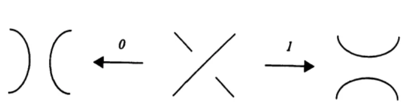
A 0-smoothing and a l-smoothing are local moves on a link diagram

as

in Figure 1. We denote by

$D_{s}$ the loops which are obtained from$D$ by applying $s_{i}$-smoothingat $c_{i}(i=1, \cdots, n)$ and by $|D_{s}|$

(2)

$rightarrow$

Figure 1: 0- and l-smoothings

and $x$

.

The object ofLee’s complex is defined

as

follows,

$\sigma_{Lee}(D)=\bigoplus_{s\in\{0,1\}^{n}}|s|=\iota^{V^{\otimes|D_{s}|}}$ and _{$C_{Lee}^{*}(D)= \bigoplus_{i\in Z}C_{Lee}^{i}(D)$}

.

The multiplication $m:V\otimes Varrow V$ and the comultiplication $\Delta$ : _{$Varrow V\otimes V$}

are

defined by

$m(1\otimes 1)=m(x\otimes x)=1$, $\Delta(1)=1\otimes x+x\otimes 1$,

$m(1\otimes x)=m(x\otimes 1)=x$

,

$\Delta(x)=x\otimes x+1\otimes 1$

.

Let $\xi=$ _{$(\xi_{1}, --, \xi_{i}, \cdots, \xi_{n})$} _be _an _{edge of the}

n-dimensional

cube $[0,1]^{n}$, that is,

an

element of

$\{0, *, 1\}^{n}$ with just

one

$*$

.

Suppose that _{$\xi_{i}=*$}

.

Then

we

define to be $|\xi|=\xi_{1}+\cdots+\xi_{i-1},$ _$\xi(0)=$

$(\xi_{1}, \cdots, \xi_{i-1},0, \xi_{i+1}, \cdots,\xi_{n}),$ _{$\xi(1)=(\xi_{1},$}

$\cdots$ $\xi_{i-1},1,$$\xi_{i+1},$

$\cdots,$$\xi_{n})$ and $\xi(*)=i$

.

For example,

suppose that $n=5$ _and$\xi=(1,1, *, 0,1)$

.

_Then $|\xi|=2,$ _{$\xi(0)=(1,1,0,0,1),$ $\xi(1)=(1,1,1,0,1)$}

and

$\xi(*)=3$

.

For

an

edge $\xi$,

we

associate the

cobordism

$S_{\xi}$ from $D$ to $D$

as

follo

neighborhood of the $\xi(*)-$th crossing, assign

a

_product

cobordism, _{and fill the saddle cobordi}

$\xi(0)$ $\xi(1)$

as

$o$

ows: we

remove

a

between

the 0- and _l-smoothings _{around the} $\xi(*)-$th crossing. The cobordism _{is either of th}

co or

lsm

following twotypes: (i) two circles of$D_{\xi(0)}$ merge into

one

circle of$D$ or (ii)

one

_{circle of}_$D$

$1Se$ler $0$ te

$\zeta(1)$, or

splits _{into two circles} _of$D_{\xi(1)}.$ Rrthermore,

we

associate the ma $d\cdot V^{\otimes|D_{\zeta(0)}|}$

$\xi(0)$

$p$ $\xi$

.

$arrow V$ $\xi(1)$

as

$\otimes|D$ $|$

follows: the

homeomorphism

$d_{\xi}$ is induced by the map

$m$ if the cobordism $S$ is of$t$

the map $\Delta$ ifthe

cobordism

$S_{\xi}$ is of type (ii).

Note

that

we

set $d$ to be the $\xi identit^{yp}n$

the ten

$y$ $e(i)$ and $b$

factors

_{corresponding to} _the _loops_{that do not participate.} _For $an\xi$

element $x\in V^{\otimes|D,|}\subset yonC_{Lee}^{i}(D)$

, $e$

ensor

we define $\theta$

as

follows,

$d^{t}(x)= \sum_{\xi\in\{0,*,1\}^{n}:\xi(0)=s}(-1)^{|\xi|}d_{\xi}(x)$,

where $s$is

a

statefor$D$

.

Let$d$be

$\oplus_{i\in Z}\theta$

.

We obtain$d^{2}=0$

.

Thecomplex_$C^{*}$

$(D)-(C^{*}$ $(D$ $d$

is called Lee’s complex. The Lee’s homology of$KH^{*}$ $(K)$, is defined _to $betheh^{-}mo1LeeLee$

$)$, $)$

of$C_{Lee}^{*}(D).$ By the following lemma,

$H_{Lee}^{*}(K)$ does $notdependLee$ on the choice of diagrams of

$K$

.

$e$ omo ogy group

Lemma 2.1 ([13]). Let$D$ and$D’$ be diagrams

of

a _knot_K. _Then

$C_{Lee}^{*}(D)$ and$C_{Lee}^{*}(D’)$ are chain

homotopic.

2.2 The

basis

of

Lee’s

homology

of

a

knot

It is known that Lee’s homology of a knotisverysimple

as

avector space. Indeed, Lee [13] _showed

that $\dim H_{Lee}^{*}(K)=2$and

described

a basis _of_{Lee’s homology}_of

_a

_knot

$K$

.

In thissubsection

_we

ee [13] showe

explain _{these results.} _We _also _recall _{the notion of}_{an enhanced} _state.

It is useful to

use

the basis $a=1+x,$ $b=1-x$ of $V$

.

Then

$m(a\otimes a)=2a,$$m(b\otimes b)=2b$, $\triangle(a)=2a\otimes a$,

(3)

For astate $s$ for $D$, wedefine col$(D_{s})$ to be the set of coloring maps from the components of$D_{s}$ to

V. Note that an element of col$(D_{s})$ is naturally identified with an element of $V^{\otimes|D_{S}|}\subset C_{Lee}^{|s|}(D)$

.

Hereafterwe always identify an element ofcol$(D_{s})$ withthe element of $V^{\otimes|D_{S}|}\subset C_{Lee}^{|s|}(D)$

.

We call

an

element of col$(D_{s})$

an

enhanced state.

Let$0$ be theorientationof$D$ and $s_{o}$ thestatefor $D$ correspondingto$0$, that is, the state whose

i-th element is $0$ ifthe sign of

$c_{i}$ is positive and 1 if the sign of$c_{i}$ is negative. Then, by definition,

$D_{s_{O}}$ arethe Seifert circles and _{$|s_{o}|=0$}

.

Let_{$f_{0}(D)\in$} col$(D_{s_{o}})$be theenhanced state whose values of

any adjacent Seifert circlesare$a$ and$b$respectively and the outer most right-handed Seifert circle is

$a$ andthe outer most left-handed Seifert circle is $b$ (seeFigure 3). Let5be thereversed orientation

of $D$

.

Then _{$f_{0}(D)$} and $f_{\overline{o}}(D)$

are

cycles of$C_{Lee}^{0}(D)$ and weobtain the following.

Theorem 2.2 ([13]). Let $K$ be a knot and $D$ a diagram

of

K. Then

$H_{Lee}^{i}(K)=\{\begin{array}{ll}\mathbb{Q}\oplus \mathbb{Q} i=0,0 i\neq 0.\end{array}$

Here, $[f_{0}(D)]$ and $[f_{\overline{o}}(D)]fom$ a basis

of

$H_{Lee}^{0}(K)$

.

Remark 2.3. The two cycles $f_{0}(D)$ and $f_{\overline{o}}(D)$ are determined up to multiplication of$2^{c}$, where _$c$

isan integer (see [13]). Therefore we call $[f_{0}(D)]$ and $[f_{\overline{o}}(D)]$ the canonical classes of$H_{Lee}^{*}(K)$

.

3 State

cycles which represent canonical classes

In this section, we recall the notion of a state cycle, which is a cycle of $C_{Lee}^{0}(D)$ and a result on

state cycles (Theorem 3.2).

We recallsome terms. A Seifert circle of adiagram is strongly negative if signs of the adjacent

crossings to it are all negative. Let $D$ be a diagram ofa knot. An enhanced state $g\in$ col$(D_{s_{o}})$ is

state cycle if$f_{0}(l)=g(l)$ for any Seifert circle $l$which is not strongly negative. We define _{$col_{o}(D_{s_{o}})$}

to be the subset of col$(D_{s_{o}})$ which consists of state cycles. Note that the cycle $f_{0}(D)$ is a state

cycle. Any state cycles are, indeed, cycles of$C_{Lee}^{0}(D)$ as follows:

Lemma 3.1 ([1]). Let $D$ be a diagram

of

a knot and$g$ astate cycle. Then$g$ is a cycle

of

$C_{Lee}^{0}(D)$

$i.e$

.

$d^{0}(g)=0$

.

In general, the homology class of a cycle of $C_{Lee}^{0}(D)$ has many representatives. Let $f_{2}(D)$ be

the state cycle such that $f_{2}(D)(l)=2$ for any strongly negativeSeifert circle $l$

.

Then weobtain the

following:

Theorem 3.2 ([1]). Let $D$ be

a

non-negative diagram

of

a knot K. Then _{$[f_{0}(D)]=[f_{2}(D)]$}

.

We give anexample which illustrates Theorem 3.2.

Example 3.3. Let $D$ be the standard pretzel diagram of $P(3, -3, -3)$

.

Figure 2 illustrates $D$,

its Seifert circles and strongly negative Seifert circles. Let $g\in C_{Lee}^{-1}(D)$ be the enhanced state as

in Figure 3. Then $f_{0}(D)-d^{-1}(g)$ is also a state cycle as in Figure 3. Let $h\in C_{Lee}^{-1}(D)$ be the

enhanced state

as

in Figure 4. Then $f_{2}(D)=f_{0}(D)-d^{-1}(g)-d^{-1}(h)$

as

in Figure 4. Therefore

(4)

$|\backslash \backslash \sim’;\backslash \text{ノ^{}\sim}\backslash ,\gamma_{/^{\wedge}}^{\prime\sim\sim_{\backslash }}.\}$ $O$ $’$ $’\backslash _{-\supset}$

$/^{\text{へ}}\backslash ^{×_{\vee}/^{-}\backslash \text{ノ^{}i}}\vee;)$

Figure 2: The standard pretzel diagram of $P(3, -3, -3)$, its Seifert circles and strongly negative

Seifert circles

$f_{0}(D)$ $g$ $-d^{-1}(g)$ $f_{0}(D)-d^{-1}(g)$

Figure 3: Some enhanced states

$f_{0}(D)-d^{-1}(g)$ $h$

$-d^{-1}(h)$ $f_{0}(D)-d^{-1}(g)-d^{-1}(h)$

Figure 4: Someenhanced states

(5)

4 The

Rasmussen

invariant

of

a

knot and the sharper slice-Bennequin

inequality

In this section, we recall the definition of the Rasmussen invariant of a knot and the sharper

slice-Bennequin inequality for the Rasmusseninvariant of aknot.

We define a grading $p$ on $V$ by setting $p(1)=1$ and $p(x)=-1$ and extend it to $V^{\otimes n}$ by

$p(v_{1}\otimes v_{2}\otimes, \cdots, v_{n})=p(v_{1})+p(v_{2})+\cdots+p(v_{n})$

.

Nextwe define afiltration grading $q$ on $C_{Lee}^{i}(D)$ by $q(v)=p(v)+i+\omega(D)$, where $v$ is a monomial of $C_{Lee}^{i}(D)$ and $\omega(D)$ is the writhe of $D$, and

extend it to $C_{Lee}^{i}(D)$ by$\min\{q(v_{j})\}$ where $v= \sum v_{j}\in C_{Lee}^{*}(D)$ and $v_{j}$ is

a

monomial. Let

$PC_{Lee}^{*}(D)=\{v\in C_{Lee}^{*}(D)\backslash \{0\}|q(v)\geq i\}\cup\{0\}$

.

Then $\{PC_{Lee}^{*}(D)\}$ is a filtration of$C_{Lee}^{*}(D)$

.

Rasmussen showed the following.

Lemma 4.1 ([19]). Let $D$ and$D’$ be diagmms

of

a knot. Then $C_{Lee}^{*}(D)$ and$C_{Lee}^{*}(D’)$ are

filtered

chain homotopic.

Wealso denote by$q$ thefiltration gradingon$H_{Lee}^{*}(K)$ whichis induced by the filtration grading

$q$ on $C_{Lee}^{*}(D)$

.

Let

$q_{\max}(K)= \max\{q(x)|x\in H_{Lee}^{*}(K), x\neq 0\}$, $q_{\min}(K)= \min\{q(x)|x\in H_{Lee}^{*}(K), x\neq 0\}$

.

The Rasmussen invariant ofa knot $K,$ $s(K)$, is define to be $\frac{q_{\max}(K)-q_{\min}(K)}{2}$

.

By Lemma 4.1,

$s(K)$ _{does not} _depend on _{the choice of diagrams of}$K$

.

Lemma 4.2 ([19]). Let $K$ be a knot and $D$ a diagram

of

K. Then

(1) $q_{\min}(K)=q([f_{0}(D)])=q([f_{\overline{o}}(D)])$

.

(2) $q_{\max}(K)-q_{\min}(K)=2$

.

Note that $s(K)$ is equalto $q([f_{0}(D)])+1$ by Lemma4.2. The following theorem is the sharper

slice-Bennequin inequalityfor the Rasmussen invariant, whichwas first proved by Kawamura [10].

Note that the state cycle in Theorem 3.2 implies the sharper slice-Bennequin inequality for the

Rasmussen invariant.

Theorem 4.3 ([1] and [10]). Let $D$ be a non-negative diagram

of

a K. Then

$w(D)-O(D)+2O_{<}(D)+1\leq s(K)$,

where $O_{<}(D)$ is the number

of

strongly negative circles

of

$D$.

5 Kawamura-Lobb

$s$

inequality

for

the

Rasmussen

invariant

Inthis section,werecallKawamura-Lobb$s$inequalityfortheRasmusseninvariant, which isstronger

than the sharper slice-Bennequin inequality, and that the equality holds for homogeneous knots.

Let $O_{+}(D)^{1}$ and $O_{-}(D)$ be the numbers of connected components of the diagrams which is

obtained from $D$ by smoothing all negative and positive crossings of $D$, respectively. Kawamura

[11] and Lobb [17] independently obtained a stronger estimation for the Rasmussen invariant as

follows:

(6)

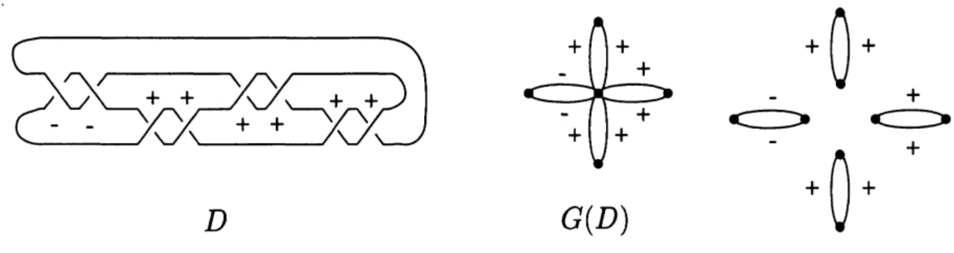
$D$ $G(D)$ $+0+$ $+$

$=$

$(ii=$

$+0+$ $+$

Figure 6: A non-alternating and non-positive diagram $D$ and the graph $G(D)$

Theorem 5.1 ([11] and [17]). Let$D$ be

a

diagram

of

a knot K. Then

$w(D)-O(D)+2O_{+}(D)-1\leq s(K)$,

where $\omega(D)$ denotes the writhe

of

$D(i.e$

.

the number

of

positive crossings

of

$D$ minus the number

of

negative cmssings

_of

$D$) and$O(D)$ denotes the number

of

the

Seifert

circles

of

$D$

.

Cromwell [5] introduced the notionofhomogeneityfor knots to generalize results

on

alternating

knots. The notion ofhomogeneity is also defined forsigned graphs and diagrams: A signed graph

is homogeneous if each block has the

same

signs, and a diagram $D$ of a knot is homogeneous

if its Seifert graph, denoted by $G(D)$, is homogeneous (for

more

details,

see

[2]). A knot $K$ is

homogeneous if$K$ has ahomogeneous diagram. In [2], we determined the Rasmussen invariant of

ahomogeneous knot

as

follows:

Theorem 5.2 ([2]). Let$D$ be a homogeneous diagmm

of

a knot K. Then

$s(K)=w(D)-O(D)+2O_{+}(D)-1$

.

6 A

criteria

on

homogeneous

knots

Inthis section, weconsider

some

homogeneous knotsandgivea new criteria

on

homogeneousknots.

Cromwell [5] showed thatalternating diagrams and positive diagrams

are

homogeneous. There

aremany homogeneous diagrams whichareneither alternatingnorpositive. The following isasuch

example.

Example 6.1. Let $D$ be the diagram

as

in Figure 6. Then $G(D)$ is homogeneous (see Figure 6).

Therefore $D$ is a homogeneous diagram whichis neither alternating nor positive.

Theclass of homogeneous knots includes alternating knots and positive knots. Another example

of a homogeneous knot is the closure of

a

homogeneous braid, a notion which

was

introduced by

Stallings [21]. Let $B_{n}$ be the braid group on $n$ strands with generators $\sigma_{1},$$\sigma_{2},$_$\cdots,$$\sigma_{n-1}$

.

A braid

$\beta=\sigma_{i_{1}}^{\epsilon_{1}}\sigma_{i_{2}}^{\epsilon 2}\cdots\sigma_{i_{k}}^{\epsilon_{k}},$$\epsilon_{j}=\pm 1(j=1, \cdots, k)$ is homogeneous if

(1) every $\sigma_{j}$ occurs at least once,

(7)

Table 1:

For example, the braid $\sigma_{1}\sigma_{2}^{-1}\sigma_{1}\sigma_{2}^{-1}$ is homogeneous, however, the braid $\sigma_{1}^{2}\sigma_{2}\sigma_{1}\sigma_{2}^{-1}$ is not

homo-geneous.

Lemma 6.2 ([5]). Let $\beta$ be a braid whose closure is a knot. Then $\beta$ is homogeneous

if

and only

if

the knot diagmm

_of

the closure

_of

$\beta$ is homogeneous.

A homogeneous bmid knot is the closure of a homogeneous braid. By the above lemma, a

homogeneous braid knot is homogeneous. The knot $9_{43}$ is a homogeneous braid knot whichis not

neither alternating nor positive.

Stallings [21] proved thata homogeneousbraid knot is fibered. Notice that there exist

homoge-neous knotswhich arenot homogeneous braid knotssince somehomogeneous knots arenot fibered

(for example, $5_{2}$). The knot $9_{49}$ is a homogeneous knot which are neither homogeneous braid,

alternating, nor positive. We give tables of non-alternating homogeneous knots and homogeneous

braid knots up to 10 crossings, respectively. The table of non-alternating homogeneous knots up

to 10 crossings isdue to Cromwell [5].

(8)

Figure 7: A diagram of$8_{19}$ and its Seifert circles

Theorem 6.3 (Theorem 1.3 in [2]). A knot $K$ is positive

if

and only

if

$K$ homogeneous and

$s(K)/2=g_{*}(K)=g(K)$, where$g_{*}(K)$ is the

4-ball

genus

of

$K$ and$g(K)$ is the genus

of

$K$

.

As

a

corollary, we obtain the following:

Corollary 6.4.

_If

$K$ is not positive and $s(K)=2g(K)$, then $K$ is not homogeneous.

This corollary gives

us

a new

method to show that

some

knots

are

not homogeneous. The

following issuch

an

example.

Example 6.5. Let $K$ bethe knot $10_{145}$

.

Then $K$ is not positive and $s(K)=2g(K)=4$ (see [4]).

Therefore $K$ is not homogeneous.

7 Non

state

cycles which represent

canonical classes

In section 3, we described state cycles which give the sharper slice-Bennequin inequality for the

Rasmussen invariant. In this section,we considercycleswhichgive Kawamura-Lobb’ inequality for

the Rasmussen invariant, which is stronger thanthe sharper slice-Bennequininequality.

First we give some examples of knot diagrams such that Kawamura-Lobb’ inequality gives a

strongerestimation than the sharper slice-Bennequin inequality.

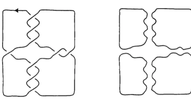
Example 7.1. Let$D$ be the diagram of$8_{19}$

as

in Figure 7. Then$\omega(D)=3,$$O(D)=4,$$O_{<}(D)=0$

and$O_{+}(D)=2$

.

Therefore the sharper slice-Bennequin inequality implies that$0=3-4+0+1\leq$

$s(8_{19})$ and Kawamura-Lobb’ inequalityimplies that $2=3-4+2+1\leq s(8_{19})$

.

Note that $s(8_{19})=2$

(see [4]).

Example 7.2. Let$D$bethe alternating diagram asinFigure8and$K$the knot which isrepresented

by $D$

.

Then _{$\omega(D)=-3,$} $O(D)=6,$_{$O_{<}(D)=2$} and _{$O_{+}(D)=4$}. Therefore the sharper

slice-Bennequin inequality implies that $-4=-3-6+4+1\leq s(K)$ and Kawamura-Lobb’ inequality

implies that $-2=-3-6+6+1\leq s(K)$

.

Since $K$ is the connected sum of two figure-eight knots

and the trefoil knot, $s(K)=-2$ (see [19]).

Next wegivesome cycles which give Kawamura-Lobb’ inequality for theRasmussen invariant.

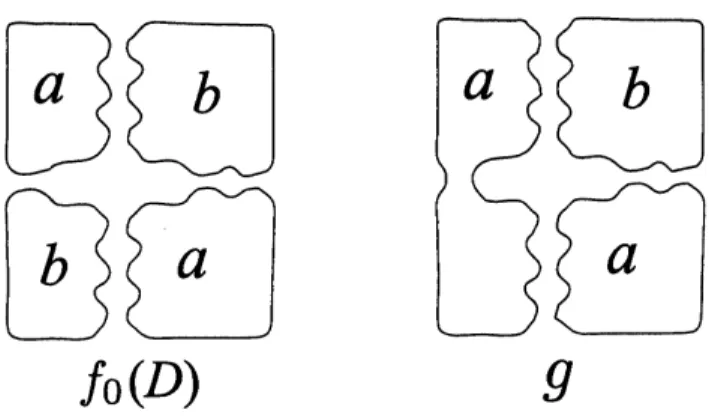
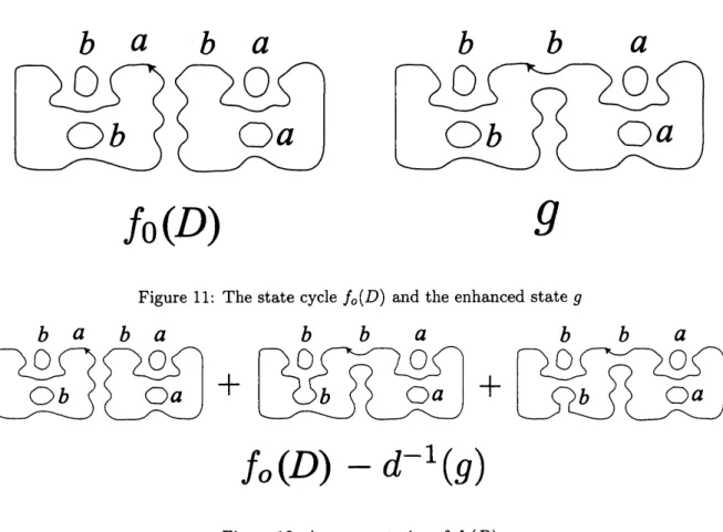
Example 7.3. Let $D$ be the diagram of $8_{19}$

as

in Figure 7. Let $g\in C_{Lee}^{-1}(D)$ be the enhanced

state

as

in Figure 9. Then $f_{0}(D)-d^{-1}(g)$ is not

a

state cycle

as

in Figure 10. Note that the cycle

(9)

Figure

8:

An alternating diagram and its Seifert circles

$f_{0}(D)$ $g$

Figure 9: The state cycle $f_{0}(D)$ and the enhanced state$g$

$b$

$+$

$2a$

$f_{0}(D)$

–

$d^{-1}(g)$

(10)

$f_{0}(D)$ $g$

Figure 11: Thestate cycle $f_{0}(D)$ and the enhanced state $g$

$b$

a

$b$

a

$f_{0}(D)$ – $d^{-1}(g)$

Figure 12: A representative of $f_{0}(D)$

Example 7.4. Let$D$bethe alternating diagram

as

inFigure8and$K$the knot which is represented

by $D$. Let $g\in C_{Lee}^{-1}(D)$ be the enhanced state

as

in Figure 11. Then $f_{0}(D)-d^{-1}(g)$ is not a state

cycle

as

inFigure 10. Notethat the cycle$f_{0}(D)-d^{-1}(g)$ impliesthat-2 $=-3-6+6+1\leq s(K)$,

which is Kawamura-Lobb’ inequality.

Problem 7.5. Let$D$ be a knot diagram. Find an explicit presentation

of

a cycle $f(D)$ such that

$[f_{0}(D)]=[f(D)]$ _{and $q(f(D))=w(D)-O(D)+2O_{+}(D)-2$ .}

In general,

even

for

an

alternating diagram $D$,

we

do not know

an

explicit presentation of a

cycle $f(D)$ such that $[f_{0}(D)]=[f(D)]$ and $q(f(D))=w(D)-O(D)+2O_{+}(D)-2$

.

8 Non

homogeneous

knots

There are many non homogeneous knots. One of them is the pretzel knot of type $(p, -q, -r)$ for

odd integer $|p|\geq 3,$ $|q|\geq 3,$ $|r|\geq 3$ (see [5]). Another example is the untwisted Whitehead double

ofa knot (see [5]). For diagrams of these knots, it

seem

to be

more

hard to describe cycles which

determine the Rasmussen invariant.

References

[1] T. Abe, State cycles which represent canonical classes

of

Lee’s homology

_of

a knot, preprint.

(11)

Figure 13: $P(3,-5,-7)$ _{and the untwisted Whitehead double} _of_the_trefoil knot

[3] Cornelia A. Van Cott, Ozsvath-Szabo and Rasmussen invamants

_of

cable knots,

arXiv:0803.0500v2 [math. GT].

[4] J. C. Cha and C. Livingston,

_KnotInfo:

Table

_of

Knot Invariants,

http:$//www$_{.indiana.edu/knotinfo,} _{July 2,} _2010.

[5] P. R. Cromwell, Homogeneous links, J. London Math. Soc. (2) 39 (1989), no. 3, 535-552.

[6] P. R. Cromwell, Knots and Links, Cambridge University Press, (2004).

[7] A. Elliott, State Cycles, Quasipositive Modification, and Constructing H-thick Knots in

Kho-vanovHomology, arXiv:0901.4039v2 [math.GT].

[8] M. Freedman, R. Gompf, S. Morrison, K. Walker, Man and machine thinking about the smooth

4-dimensional

Poincare conjecture,arXiv:0906.5177v2 [math.GT].

[9] M. Hedden and P. Ording, The $Ozsv\acute{a}th-Szab\mathscr{E}$andRasmussen concordance invart,ants are not

equal, Amer. J. Math. 130 (2008), no. 2, 441-453.

[10] T. Kawamura, The Rasmusseninvareants and the sharperslice-Bennequininequality on knots,

Topology46 (2007), no. 1, 29-38.

[11] T. Kawamura, An estimate

_of

the Rasmussen invariant

_for

links, preprint (2009).

[12] M. Khovanov, A categorification

_of

the Jones polynomial, Duke Math. J. 101 (2000), no. 3,

359-426.

[13] E. S. Lee, An endomorphism

_of

the Khovanov invariant, Adv. Math. 197 (2005),

no.

2,

554-586.

[14] C. Livingston, Computations

_of

the Ozsvath-Szabo knot concordance invariant, Geom. Topol.

8 (2004) 735-742.

[15] C. Livingston and S. Naik, Ozsvath-Szabo andRasmussen invariants

_of

doubledknots, Algebr.

Geom. Topol. 6 (2006), 651-657.

[16] C. Livingston, Slice knots with distinct Ozsvath-Szab6 andRasmussen invariants, Proc. Amer.

Math. Soc. 136 (2008), no. 1, 347-349.

[17] A. Lobb, Computable bounds

_for

Rasmussen’s concordance invanant, arXiv:0908.2745v2

(12)

[19] J. Rasmussen, Khovanov homology and the slice genus, to appear in Invent. Math.

[20] A. Shumakovitch, Rasmussen invariant, slice-Bennequin inequality, and sliceness

of

knots

math, J. Knot Theory Ramifications 16 (2007), no. 10, 1403-1412.

[21] J. Stallings, Constructions

_{of fibred}

knots and links, Algebraic and geometric topology (Proc.

Sympos. Pure Math., Stanford Univ., Stanford, Calif., 1976),Part 2, pp. 55-60, Proc. Sympos.

Pure Math., XXXII, Amer. Math. Soc., Providence, R. I., 1978.

[22] A. Stoimenow,

Some

examples related to knotsliceness,

J.

Pure Appl. Algebra 210 (2007),

no.

1,

161-175.

[23] S. Wehrli, Contributions to Khovanov Homology, arXiv:0810.0778.

[24] S. Wehrli, Catego

_{rification of}

the colored Jones polynomial and Rasmussen invariant

_of

links,

Canad. J. Math. 60 (2008), no. 6, 1240-1266.