Some
computer
assisted
proofs
on
the
bifurcation
structure
of solutions for the
Rayleigh-B\’enard problem
九州大学情報基盤センター
渡部善隆
(Yoshitaka Watanabe)
Computing and
Communications
Center,
Kyushu
University
1
The Rayleigh-Benard
problem
Consider a plane horizontal layer (see Figure 1) ofan incompressible viscous fluid
heated fromthe bottom. At the lowerboundary: $z=0$ the layerof fluid ismaintained
at temperature $T+\delta T$ and the temperature ofthe upper boundary $(z=h)$ is $T$
.
Figure 1. Model of fluid layer
As well known, under the vanishingassumption in$y$-direction, the two-dimensional
(x-z) heat convection model can be described
as
the following Oberbeck-Boussinesqapproximations $[1, 3]$: $u_{t}+uu_{x}+wu_{z}$ $=$ $p_{x}+P\Delta u$, $w_{t}+uw_{x}+ww_{z}$ $=$ $p_{z}-P\mathcal{R}\theta+P\Delta w$, (1) $u_{x}+w_{z}$ $=$ $0$, $\theta_{t}+w’+u\theta_{x}+w\theta_{z}$ $=$ $\Delta\theta$
.
Here, $u$ and $w$
are
velocity in $x$ and $z$, respectively, $p,$ $\theta$are
pressure and temper-ature field reprensating deviation from the linear profile, $*\epsilon:=\partial/\partial\xi(\xi=x, z, t),$ $\Delta:=$ $\partial^{2}/\partial x^{2}+\partial^{2}/\partial z^{2},$ $\mathcal{R}$ isRayleigh number and $\mathcal{P}$ is Prandtl number.In previous results$[8, 9]$, the authors considered the Rayleigh-B\’enard problem (1)
and proposed an approachto prove the exsistence ofthe steady-state solutions based on the infinite dimensional fixed-point theorem using Newton-like operator with the spectral approximation and the constructive error estimates. For the given Prandtl and Rayleigh numbers, several exact non-trivial solutions have been verified.
This paper will present
a
computer assisted proof of the existence fora
symmetry-breaking bifurcation point which is an important information to clarify the globalbifurcation structure.
2
Fixed-point
formulation
of problem
This section describes
on a
basic concept ofour numerical verification method to prove the exsistence of the steady-state solutions. Since we only consider the thesteady-state solutions, $u_{t},$ $w_{t}$ and $\theta_{t}$ vanish in (1). And also
assume
that all fluid motion is confined to the rectangular region$\Omega:=\{0<x<2\pi/a, 0<z<\pi\}$
for
a
givenwave
number $a>0$.
Let us impose periodic boundary condition (period $2\pi/a$) in the horizontal
direc-tion, stress-free boundary conditions $(u_{z}=w=0)$ for the velocity field and Dirichlet boundaryconditions $(\theta=0)$ forthetemperature fieldon thesurfaces $z=0,$$\pi$,
respec-tively. liurthermore, we assume the following evenness and oddness conditions [2]: $u(x, z)=-u(-x, z)$, $w(x, z)=w(-x, z)$, $\theta(x, z)=\theta(-x, z)$
.
We use the stream function $\Psi$ satisfying
$u=-\Psi_{z}$, $w=\Psi_{x}$
so that $u_{x}+w_{z}=0$
.
By some simple calculations in (1) with setting $\Theta:=\sqrt{P\mathcal{R}}\theta$,we obtain
$P\Delta^{2}\Psi$ $=$ $\sqrt{P\mathcal{R}}\Theta_{x}-\Psi_{z}\Delta\Psi_{x}+\Psi_{x}\Delta\Psi_{z}$,
(2)
$-\Delta\Theta$ $=$ $-\sqrt{P\mathcal{R}}$$\Psi_{x}+\Psi_{z}\Theta_{x}$ $-\Psi_{x}\Theta_{z}$
.
IFMrom the boundary conditions, the functions V and $\Theta$ can be assumed tohave the
following double Fourier series:
We now define the following function spaces for integers $k\geq 0$:
$X^{k}:= \{\sum_{m=1}^{\infty}\sum_{n=1}^{\infty}A_{mn}\sin(amx)\sin(nz)|A_{mn}\in \mathrm{R}$, $\sum_{m=1}^{\infty}\sum_{n=1}^{\infty}((am)^{2k}+n^{2k})A_{mn}^{2}<\infty\}$ ,
$\mathrm{Y}^{k}:=\{$$\sum_{m=0}^{\infty}\sum_{n=1}^{\infty}B_{mn}\cos(amx)\sin(nz)|B_{mn}\in \mathrm{R}$, $\sum_{m=0}^{\infty}\sum_{n=1}^{\infty}((am)^{2k}+n^{2k})B_{mn}^{2}<\infty\}$ .
In order to get the enclosure of the exact solutions for the problem (2), we need
some
appropriate finite dimensional subspaces. For $M_{1},$ $N_{1},$$\Lambda\prime I_{2}\geq 1$ and $N_{2}\geq 0$, weset $N:=(M_{1}, N_{1}, M_{2}, N_{2})$ and define the finite dimensional approximate subspaces by
$S_{N}^{(1)}:= \{\Psi_{N}=\sum_{m=1}^{M_{1}}\sum_{n=1}^{N_{1}}\hat{A}_{mn}\sin(amx)\sin(nz)|\hat{A}_{mn}\in \mathrm{R}\}$ ,
$S_{N}^{(2)}:= \{\Theta_{N}=\sum_{m=0}^{M_{2}}\sum_{n=1}^{N_{2}}\hat{B}_{mn}\cos(amx)\sin(nz)|\hat{B}_{mn}\in \mathrm{R}\}$ ,
$S_{N}:=S_{N}^{(1)}\mathrm{x}S_{N}^{(2)}$
.
Let denote an approximate solution of(2) by $\hat{u}_{N}:=(\hat{\Psi}_{N},\hat{\Theta}_{N})\in S_{N}$
.
We now set $f_{1}(\Psi, \Theta)$ $:=$ $\sqrt{P\mathcal{R}}\Theta_{x}-\Psi_{z}\Delta\Psi_{x}+\Psi_{x}\Delta\Psi_{z}$,$f_{2}(\Psi,\ominus):=-\sqrt{\mathcal{P}\mathcal{R}}\Psi_{x}+\Psi_{z}\Theta_{x}-\Psi_{x}\Theta_{z}$,
where
$\Psi=\hat{\Psi}_{N}+w^{(1)}$, $\Theta=\hat{}_{N}+w^{(2)}$.
Then the problem (2) is rewritten as the following system ofequations with respect to $(w^{(1)}, w^{(2)})\in X^{4}\cross \mathrm{Y}^{2}\mathrm{s}\mathrm{a}\mathrm{t}\mathrm{i}\mathrm{s}\theta$ing
$\mathcal{P}\Delta^{2}w^{(1)}=f_{1}(\hat{\Psi}_{N}+w^{(1)},\hat{\Theta}_{N}+w^{(2)})-P\Delta^{2}\hat{\Psi}_{N}$,
$-\Delta w^{(2)}=f_{2}(\hat{\Psi}_{N}+w^{(1)},\hat{\Theta}_{N}+w^{(2)})+\Delta\hat{\Theta}_{N}$, (4)
which is so-called a residual form. Setting
$w$ $=$ $(w^{(1)}, w^{(2)})$,
$h_{1}(w)$ $=$ $f_{1}(\hat{\Psi}_{N}+w^{(1)},\hat{\Theta}_{N}+w^{(2)})-P\Delta^{2}\hat{\Psi}_{N}$ ,
$h_{2}(w)$ $=$ $f_{2}(\hat{\Psi}_{N}+w^{(1)},\hat{\Theta}_{N}+w^{(2)})+\Delta\hat{\Theta}_{N}$,
by virtue of the Sobolev embbeding theorem and the definition of $f_{1}$ and $f_{2},$ $h$ is
a
bounded continuousmap from $X^{3}\cross \mathrm{Y}^{1}$ to$X^{0}\cross \mathrm{Y}^{0}$. Moreover, itis easilyshown that for all $(g_{1}, g_{2})\in X^{0}\cross \mathrm{Y}^{0}$, the linear problem:
$\Delta^{2}\overline{\Psi}$
$=$ $g_{1}$, $-\Delta\overline{\Theta}$
$=$ $g_{2}$
(5)
has
a
unique solution $(\overline{\Psi},\overline{\Theta})\in X^{4}\cross \mathrm{Y}^{2}$.
We denote this mapping by $\overline{\Psi}=(\Delta^{2})^{-1}g_{1}$ and $\overline{\Theta}=(-\Delta)^{-1}g_{2}$, then the operator:$\mathcal{K}:=(P^{-1}(\Delta^{2})^{-1}, (-\Delta)^{-1}):X^{0}\cross \mathrm{Y}^{0}arrow X^{3}\cross \mathrm{Y}^{1}$
is
a
compact map because of the compactness of the imbedding $X^{4}arrow X^{3}$ and$\mathrm{Y}^{2}arrow \mathrm{Y}^{1}$ and theboundedness of $(\Delta^{2})^{-1}$ : $X^{0}arrow X^{4},$ $(-\Delta)^{-1}$ : $\mathrm{Y}^{0}arrow \mathrm{Y}^{2}$
.
Thus, (4)is rewritten by a fixed-point equation:
$w=Fw$ (6)
for the
conipact
operator $F:=\mathcal{K}\mathrm{o}h$ on$X^{3}\cross \mathrm{Y}^{1}$.
Therefore, by the Schauderfixed-point theorem, ifwefind a nonempty, closed, bounded and
convex
set $W\subset X^{3}\cross \mathrm{Y}^{1}$,$\mathrm{s}\mathrm{a}\mathrm{t}\mathrm{i}\mathrm{s}\Phi \mathrm{i}\mathrm{n}\mathrm{g}$
$FW\subset W$ (7)
then there exists a solution of (6) in $W$
.
The set $W$ in (7) is referred asa
candidateset ofsolutions.
The candidate set $W$ is usually constructed by computer as a direct sum of the
finite dimensionalsubset
$W_{N}\subset S_{N}^{(1)}\mathrm{x}S_{N}^{(1)}\subset X^{3}\cross \mathrm{Y}^{1}$
and its orthogonal complement $W_{N}^{\perp}$ in the space $X^{3}\cross \mathrm{Y}^{1}$
.
By using anappropriate
projection $P_{N}$ : $X^{3}\cross \mathrm{Y}^{1}arrow X_{N}^{3}\cross \mathrm{Y}_{N}^{1}$, thedecomposed form$P_{N}FW\subset W_{N}$ and
(I-$P_{N})FW\subset W_{N}^{\perp}$ are numerically verified insteadof (7), which implies the verification
of a sufficient condition for (7). Here, the former condition is verified by direct
computation in the computer, and the latter criterion can be proved by the
effective
use of the constructive error estimates for the projection. In the present case, the projection $P_{N}$ can be taken as the finite trunction operator of solutions to (5)[8].Furthermore, in general, a kind of Newton-type formulation is utilized so that the
concerning operatorhasthe retraction property in a neighborhood of thesolution(see,
By using the Newton-like procedure [6], we succeeded to verify various kinds of bifurcating solutions as shown in Figure 2. Here, $\mathcal{R}_{C}$ implies the critical Rayleigh
number which equals 6.75. The vertical axis stands for the absolute value of the
coefficient of the approximate solution for $\Theta$
.
And each dot in Figure 2 means thatthe existenceofanexact solutioncorresponding to the point
was
numerically verified.$arrow R/\mathcal{R}_{C}$
Figure 2. Verified bifurcating solutions
3
Existence
of
bifurcation
point
Rom the observation of Figure2, particularly the behaviour around the part
en-closed by the circle, we expected that there should exists a secondary bifurcation point. Namely, near “the biffircation-like point” we found the following two different kinds ofapproximate solutions. For approximate solutions of the form
$\Psi_{N}=\sum_{m=1}^{hI_{1}}\sum_{n=1}^{N_{1}}A_{mn}\sin(amx)\sin(nz)$,
we
have following two solutions satisfying$\Theta_{N}=\sum_{m=0}^{M_{2}}\sum_{n=1}^{N_{2}}B_{mn}\cos(amx)\sin(nz)$,
$A_{mn}=B_{mn}=0$, $m=1,3,5,7,$$\ldots$with$\mathcal{R}=32$
and
$A_{mn}\neq 0$, $B_{mn}\neq 0$, $m=1,3,5,7,$ $\ldots$with $R=33$
.
These approximate results strongly suggest that there should exist
a
In order to obtain the enclosure ofthe bifurcation point, we set and an operator
$S:X^{0}\cross \mathrm{Y}^{0}arrow X^{0}\cross \mathrm{Y}^{0}$ by
$Su=S(\Psi, )$ $=(S_{1}\Psi, S_{2})$
$=(\Psi(x+\pi/a, z),$$\Theta(x+\pi/a, z))$,
then using this “symmetric” operator $S,$ $X^{k}$ and $\mathrm{Y}^{k}$ can be decomposed as $X^{k}=X_{s}^{k}\oplus X_{a}^{k}$, $\mathrm{Y}^{k}=\mathrm{Y}_{s}^{k}\oplus \mathrm{Y}_{a}^{k}$,
where
$X_{s}^{k}=\{\Psi\in X^{k}|S_{1}\Psi=\Psi\}$, $X_{a}^{k}=\{\Psi\in X^{k}|S_{1}\Psi=-\Psi\}$,
$\mathrm{Y}_{s}^{k}=\{\Theta\in \mathrm{Y}^{k}|S_{\mathit{2}}\Theta=\}$, $\mathrm{Y}_{a}^{k}=\{\Theta\in \mathrm{Y}^{k}|S_{2}\Theta=-\Theta\}$
.
Also, setting$Z:=X^{3}\cross \mathrm{Y}^{1}$, $G:=I-F$,
$SGw=GSw$ holds and $Z$ is decomposed as
$Z=Z_{s}\oplus Z_{a}$,
where $Z_{s}=\{w\in Z;Sw=w\}$ and $Z_{a}=\{w\in Z;Sw=-w\}$
.
Next, considering $\mathcal{R}$as a
variable, let$\mathcal{G}$ be
a
mapon
$Z_{\epsilon}\cross Z_{a}\cross \mathrm{R}$defined by$\mathcal{G}(w, v, \mathcal{R}):=$
.
(8)Here $\mathcal{L}$ is
an
appropriate functionalon
$Z_{a}$
.
Then the following Lemma presented by Kawanago [4] can be applied.Lemma 1 $(w_{0}, \mathcal{R}_{0})\in Z_{\mathit{8}}\cross \mathrm{R}$isasymmetry-breaking bifurcationpoint of$G(w, \mathcal{R})=$ $0$ if
1. Extended system $\mathcal{G}(w, v, \mathcal{R})=0$ has
an
isolated solution $(w0, v_{0}, \mathcal{R}_{0})\in Z_{s}\cross$$Z_{a}\cross$ R.
2. $D_{u}G[w_{\mathit{0}}, \mathcal{R}_{0}]|_{X_{*}^{4}\mathrm{x}Y_{\epsilon}^{2}}$ : $X_{s}^{4}\mathrm{x}\mathrm{Y}_{\epsilon}^{2}arrow X_{\mathit{8}}^{0}\cross \mathrm{Y}_{\epsilon}^{0}$isbijective.
First, we tried to prove that the extended system $\mathcal{G}(w, v, \mathcal{R})=0$ has an isolated
solution $(w_{0}, v_{0}, \mathcal{R}_{0})\in Z_{s}\cross Z_{a}\cross \mathrm{R}$ by a computer-assisted approach using our ver-ification principle in the section 2. The equation $\mathcal{G}(w, v, \mathcal{R})=0$
means
the problem to find out$\mathrm{s}\mathrm{a}\mathrm{t}\mathrm{i}\mathrm{s}\wp$ing
$\mathcal{P}\Delta^{\mathit{2}}\Psi-\sqrt{\mathcal{P}\mathcal{R}}\Theta_{x}-J(\Psi, \Delta\Psi)$ $=$ $0$,
$-\Delta+\sqrt{P\mathcal{R}}\Psi_{x}+J(\Psi, )$ $=$ $0$,
$P\Delta^{2-}---\sqrt{P\mathcal{R}}^{l}\mathrm{r}_{x}-J(\Psi, \Delta_{-}^{-}-)-J(---, \Delta\Psi)$ $=$ $0$, $-\Delta^{l}\mathrm{r}+\sqrt{\mathcal{P}\mathcal{R}}---x+J(\Psi, \prime \mathrm{r})+J(_{-}^{-}-, \Theta)$ $=$ $0$,
$\mathcal{L}(v)-1$ $=$ $0$
.
(9)
Setting the functional $\mathcal{L}$ by
$\mathcal{L}(v)=(_{-,-0}^{--}--)_{L^{2}}+(’\mathrm{r}, \prime \mathrm{r}_{0})_{L^{2}}$, $—0:= \frac{2a}{\pi^{2}}\sin(ax)\sin(z)$, $\prime \mathrm{r}_{0:=}\frac{2a}{\pi^{2}}\cos(ax)\sin(z)$, denotinga fixed approximatesolutionof(9) by $[\Psi_{N}, \Theta_{N,-N}--, \prime \mathrm{r}_{N}, R_{N}]$ andusing the residual variables defined by
$\Psi=\Psi_{N}+u^{(1)},$ $\Theta=\Theta_{N}+u^{(\mathit{2})},$ $—=_{-N+u^{(3)}}--,$ $\prime \mathrm{r}=\mathrm{r}_{N+u^{(4)}}’,$ $\mathcal{R}=\mathcal{R}_{N}+u^{(5)}$,
equation (9)
can
be rewrittenas
$\mathcal{P}\Delta^{2}u^{(1\rangle}$
$=$ $\sqrt{P(R_{N}+u^{(5)})}(\Theta_{N}+u^{(2)})_{x}+J(\Psi_{N}+u^{(1}),$ $\Delta(\Psi_{N}+u^{(1)}))-P\Delta^{2}\Psi_{N}$, $-\Delta u^{(2)}$ $=$ $-\sqrt{P(R_{N}+u^{(5)})}(\Psi_{N}+u^{(1)})_{x}-J(\Psi_{N}+u^{(1)}, \Theta_{N}+u^{(2)})+\Delta\Theta_{N}$,
$\mathcal{P}\Delta^{2}u^{(3)}$ $=$ $\sqrt{P(R_{N}+u^{(5)})}(’\mathrm{r}_{N}+u^{(4)})_{x}+J(\Psi_{N}+u^{(1)}, \Delta(_{-N}^{-}-+u^{(3)}))$
$+J(_{-N}^{-}-+u^{(3)}, \Delta(\Psi_{N}+u^{(1)}))-P\Delta^{2-}--N$,
$-\Delta u^{(4)}$ $=$ $-\sqrt{P(R_{N}+u^{(5)})}(_{-N}^{-}-+u^{(3)})_{x}-J(\Psi_{N}+u^{(1)\prime},\mathrm{r}_{N}+u^{(4)})$ $-J(_{-N}^{-}-+u^{(3)}, \Theta_{N}+u^{(2)})+\Delta’\mathrm{r}_{N}$,
$u^{(5)}$ $=$ $-(_{-N}^{-(3)-}-+u, --0)_{L^{2}}-(1_{N}+u^{(4)\prime},\mathrm{r}_{0})_{L^{2}}+1+u^{(5)}$
.
(10)
We now define the nonlinear function of$\mathrm{u}:=(u^{(1)}, u^{(2)}, u^{(3)}, u^{(4)}, u^{(5)})$ by
$h_{1}(\mathrm{u}):=\sqrt{P(R_{N}+u^{(5)})}(\Theta_{N}+u^{(2)})_{x}+J(\Psi_{N}+u^{(1)}, \Delta(\Psi_{N}+u^{(1)}))-\mathcal{P}\Delta^{2}\Psi_{N}$, $h_{2}(\mathrm{u}):=-\sqrt{\mathcal{P}(R_{N}+u^{(5)})}(\Psi_{N}+u^{(1)})_{x}-J(\Psi_{N}+u^{(1)}, \Theta_{N}+u^{(2)})+\Delta\Theta_{N}$ , $h_{3}(\mathrm{u}):=\sqrt{P(R_{N}+u^{(5)})}(’\mathrm{r}_{N}+u^{(4)})_{x}+J(\Psi_{N}+u^{(1)}, \Delta(_{-N}^{-}-+u^{(3)}))$ $+J(_{-N}^{-}-+u^{(3)}, \Delta(\Psi_{N}+u^{(1)}))-P\Delta^{2-}--N$, $h_{4}(\mathrm{u}):=-\sqrt{\mathcal{P}(R_{N}+u^{(5)})}(_{-N}^{-}-+u^{(3)})_{x}-J(\Psi_{N}+u^{(1)\prime},\mathrm{r}_{N}+u^{(4)})$ $-J(_{-N}^{-}-+u^{(3)}, \Theta_{N}+u^{(2)})+\Delta’\mathrm{r}_{N}$, $h_{5}(\mathrm{u}):=-(_{-N}--+u(3),---0)_{L^{2}}-(’\mathrm{r}_{N}+u^{(4)\prime},\mathrm{r}_{0})_{L^{2}}+\beta+u^{(5)}$,
Furthermore, defining
$\mathcal{K}:=(P^{-1}(\Delta^{2})^{-1}, (-\Delta)^{-1},$$P^{-1}(\Delta^{\mathit{2}})^{-1},$$(-\Delta)^{-1},$ $I)$, $\mathcal{H}:=\mathcal{K}h$,
the equation (10)
can
be representedas
the fixedequation:$\mathrm{u}=\mathcal{H}\mathrm{u}$
on
$Z_{s}\cross Z_{a}\cross$ R. We applieda
numerical verification method basedon
Banach’s fixed-point theorem$[7, 10]$ incorporated with the interval arithmeticon
Sun ONEStudio 7 Compiler Collection Fortran 95 on FUJITSU PRIMEPOWER850 (CPU:
$\mathrm{S}\mathrm{P}\mathrm{A}\mathrm{R}\mathrm{C}64\mathrm{V}1.35\mathrm{G}\mathrm{H}\mathrm{z},$ $\mathrm{O}\mathrm{S}$: Solaris8), and proved that
there exists an isolated solution of$\mathcal{G}(w_{0}, v_{0}, \mathcal{R}_{0})=0$
.
Here$\mathcal{R}_{0}\in 32.04265510708193+[-2.910, 2.910]$ $\cross 10^{-10}$.
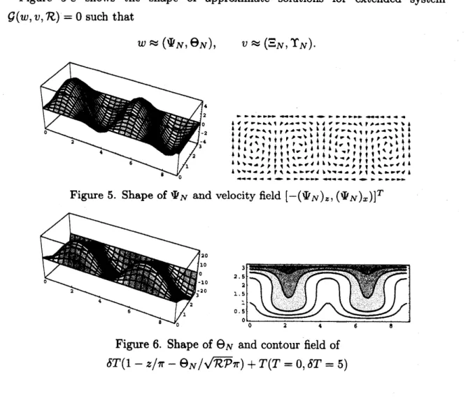
Figure 5-8 shows the shape of approximate solutions for extended system $\mathcal{G}(w, v, \mathcal{R})=0$such that
$w\approx(\Psi_{N}, \Theta_{N})$, $v\approx(_{-N}^{-\prime}-,\mathrm{r}_{N})$.
$\mathrm{F}\mathrm{i}_{1}\mathrm{r}\mathrm{e}5$. Shape of $\Psi_{N}$ and velocity field $[-(\Psi_{N})_{z}, (\Psi_{N})_{x})]^{T}$
Figure
6.
Shape of$_{N}$ and contour field ofFigure 7. Shape $\mathrm{o}\mathrm{f}_{-N}^{-}-$ and velocity field $[-(_{-N}^{-}-)z, (_{-x}^{-}-)]^{T}$
$\mathrm{F}\mathrm{i}_{1}\mathrm{r}\mathrm{e}8$. Shape of$\prime \mathrm{r}_{N}$ and contour field of
$\delta T(1-z/\pi-\prime \mathrm{r}_{N}/\sqrt{\mathcal{R}P}\pi)+T(T=0.\delta T=5)$
Therefore, from the bifurcation theorem, it implies that there exists an actual bi-furcation point in this interval if $D_{w}G[w_{0}, \mathcal{R}_{0}]$ is invertible on $Z_{s}$.
On the other hand, from the Redholm alternative, the invertibility of$D_{w}G[w_{0}, \mathcal{R}_{0}]$ is aesured when
$\mathcal{P}\Delta^{2-}---\sqrt{\mathcal{P}R_{0}}\prime \mathrm{r}_{x}-J(\Psi_{0}, \Delta_{-}^{-}-)-J(_{-}^{-}-, \Delta\Psi_{0})$ $=$ $0$, $-\Delta’\mathrm{r}+\sqrt{P\mathcal{R}_{0}}^{-_{x}}--+J(\Psi_{0}, \prime \mathrm{r})+J(_{-}^{-}-, \Theta_{0})$ $=$ $0$
has a unique trivial solution $[_{-}^{-\prime}-,\mathrm{r}]=[0,0]$ in $Z_{\theta}$, where $w_{0}=[\Psi_{0}, \Theta_{0}]$
.
We actuallysucceeded in theverificationofthe invertibility by using amethod similar to that an eigenvalue excluding technique [5]. Thus, it was numerically proved that there exists
a symmetry-breaking bifurcation point inthe above interval. References
[1] Chandrasekhar, S. (1961), Hydrodynamic and Hydromagnetic Stability, Oxford University Press.
[2] Curry, J.H. (1979), “Bounded solutions of finite dimensional approximations to
[3] Getling,A.V. (1998), Rayleigh-B\’enard Convection: structures and dynamics,
Ad-vanced series in nonlinear dynamics Vol.11, World Scientific.
[4] Kawanago, T. (2004), “A symmetry-breaking bifurcation theorem and some
re-latedtheorems applicableto maps having unbounded derivatives”, Japan Journal of Industrial and Applied Mathematics, Vol.21, pp.57-74.
[5] Nagatou, K., Yamamoto, N. and Nakao, M.T. (1999), “An approach to the
nu-merical verification of solutions for nonlinearelliptic problems withlocal
unique-ness”, Numerical Functional Analysis and Optimization, Vol.20, pp.543-565.
[6] Nakao, M.T. (2001), “Numerical verification methods for solutions of ordinary
and partialdifferential equations”, Numerical Rnctional Analysisand
Optimiza-tion, Vol.22,
No.3&4,
pp.321-356.[7] Nakao, M.T., Hashimoto, K. and Watanabe, Y. (2005), “A numerical method to Verify the invertibility of linear elliptic operators with applications to nonlinear problems”, Computing, Vol.75, pp.1-14.
[8] Watanabe, Y., Yamamoto, N., Nakao, M.T. andNishida, T. (2004), “Anumerical
verification of nontrivial solutions for the heat convection problem”, Journal of Mathematical Fluid Mechanics, Vol.6, No.1, pp.1-20.
[9] Nakao, M.T., Watanabe, Y., Yamamoto, N., Nishida, T. (2003), “Some
com-puter assisted proofs for solutions of the heat convection problems”, Reliable Computing, Vol.9, No.5, pp.359-372.
[10] Yamamoto, N. (1998), “A numerical verificationmethod for solutions of
bound-ary value problems with local uniqueness by Banach’s fixed point theorem”,


![Figure 7. Shape $\mathrm{o}\mathrm{f}_{-N}^{-}-$ and velocity field $[-(_{-N}^{-}-)z, (_{-x}^{-}-)]^{T}$](https://thumb-ap.123doks.com/thumbv2/123deta/6000799.1062235/9.892.120.769.144.658/figure-shape-mathrm-mathrm-n-velocity-field-n.webp)
