A PARABOLIC FREE BOUNDARY PROBLEM WITH BERNOULLI TYPE CONDITION ON THE FREE BOUNDARY(Variational Problems and Related Topics)

A PARABOLIC FREE BOUNDARY PROBLEM WITH

_B.ERNOULLI

TYPE CONDITION ON THE FREE BOUNDARY

JOHN ANDERSSONAND GEORG S. WEISS

ABSTHACT. Inthe brilliant paper [1], H.W Alt aiidL.A. Caffarelli provedthatcloseto

flat points the hee boundary of ccrtain weriksolutious ofthc Bernoulli $\theta \mathrm{c}.\mathrm{e}$ boundary

problem

$\Delta u-Q_{t}u=0$in $\{u>0\},$ $|\nabla u|=1$ on$\partial\{u>0\}$

.

isanalytic.

The result is related to the theory of harmonic$\mathrm{m}\mathrm{e}u$urae (see [10], [11], [12]).

For arealistic class ofsolutions, containingforexample alllimitsofthesingular

pertur-bationproblem

$\Delta u_{e}-\partial_{t}u_{e}=\beta_{e}(u_{\iota})$ as$\epsilonarrow 0$,

weprove that one-sided flatnessofthe freeboundary implies regularity.

Inparticular, weshow thatthe topologicaifree boundary $\theta\{u>0\}_{\backslash }$canbedecomposed

intoan openregular set (relative to $\partial\{u>0\}$) which is locally asurface with

H\"older-continuous spacenormal, anda closed singularset.

Ourresult extends the main theorem in the paper byH.W. Alt-L.A. $C$affarelli (1981)

to more generalsolutions as well as thetime-dependent case. Our proofuses methods

developedinH.W. Alt-L.A. Caffarelli (1981),howeverwereplacethecoreof thatpaper,

whichrelies on non-positi.ve mean curvature at singular points, by an argument based

onscaling discrepancies,whichpromisesto beapplicable to moregeneralfreeboundary

orfreediscontinuity problems.

1. INTRODUCTION

This notecontains $\mathrm{t}$ announcement

as

well as heuristics for the paper with the

same

titleto appear, but norigorous proofs. The parabolic free boundary problem

(11) $\Delta u-\partial_{t}u=0$ in _$\{u>0\},$ $|\nabla u|=1$

on

$\partial\{u>0\}$

2000 $MaV\kappa matics$Subject Classtfication. _Primary$35\mathrm{R}B5$, Secondary $35\mathrm{K}55$

.

Key words andphrases. Free boundary,BeaouUitype, parabolic,regularity, flatnessimprovement.

J. Andersson has been prtiaUysupported byafellowshipofthe${\rm Max}$Planck Society. G.S. Weiss has

been partially supported by theGrant-in-Aid 15740100/18740086of the Japanese MinistryofEducation,

Culture, Sports, Science and Ilechnology and partially supported by a fellowship of the ${\rm Max}$ Planck

Society. Bothauthors thank the$\mathrm{M}\alpha$Planck InstituteforMathematics in the Sciences for the hospitality

has $\mathrm{o}\mathrm{r}\mathrm{i}\mathrm{g}\mathrm{i}\mathrm{n}\mathrm{a}\mathrm{l}\mathrm{i}_{\mathrm{y}}$been derived as singular limit $\mathrm{h}\mathrm{o}\mathrm{m}$

a

model for the propagation of

equidif-fusional premixed flameswith high activation energy ([3]); here$u=\lambda(T_{c}-T),$ $T_{\mathrm{c}}$ is the

flame temperature, which is assumed to be constant, $T$ is the temperature outside the

flame and A is a normalization factor.

Let usshortly summarize the mathematical results directly relevantinthiscontext, begin-ningwiththe

limit

problem (1.1): in

the

brilliant paper [1], H.W. Alt and L.A. Caffarelli

proved via minimization ofthe energy $\int(|\nabla u|^{2}+\chi\{\mathrm{u}>0\})$ -here _{$\chi\{u>0\}$} denotes the

char-acteristic hiction of the set $\{u>0\}$ –existence of

a

stationary solution of (1.1) in the

sense.of

distributions. Theyako derived regularityof thehee boundary$\partial\{u>0\}$ up to

a

set ofvanishing $n-1$-dimensionalHausdorff

measure.

By [16] existence ofsingular min-imizers implies the existence of singular minimizing

cones.

L.A. Caffalelli-D. Jerison-C.

Kenigshowed thatsingular minimizing

cones

donot exist in dimension3 ([6]). Moreover itis known thatsingular minimizing

cones

exist for$n\geq 7([9])$

.

Non-minimizingsingular

cones

appearakeadyfor$n=3$ (see [1, example 2.7]). Moreoverit isknown, that solutions of the Dirichlet problem intwo space dimensions are not unique (see [1, example 2.6]).

C.E. Kenig-T. Toro ([10], [11], [12]) extended the

result

in

[1] to VMO-coefficients and

applied it to

abstract

harmonic

measures.

For

the time-dependent (1.1), both “trivialnon-uniqueness” (the positive solution of the heat equation is always another solution of (1.1)$)$ and

“non-triviaJ.

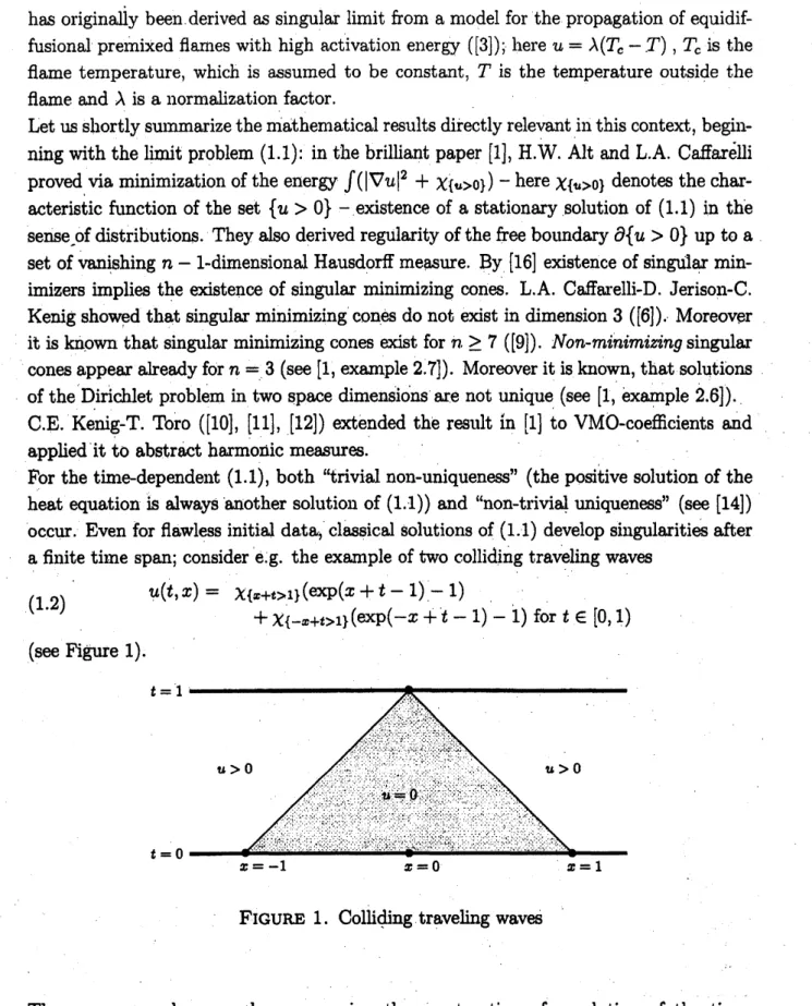
uniqueness” (see [14])

occur. Even for flawlessinitial data, classical solutions of (1.1) develop singularitiesafter

a finite time span; consider e.g. the example of two collidingtraveling

waves

$u(t,x)=\chi\{x+t>1\}(\exp(x+t-1)-1)$ (1.2)

$+\chi\{-x+t>1\}(\exp(-x+t-1)-1)$ for $t\in[0,1)$

(see Figure 1).

FIGURE 1. Colliding $\mathrm{t}\mathrm{r}\mathrm{a}\mathrm{v}\mathrm{e}1_{\dot{\mathrm{i}}}\mathrm{g}$

waves

There

are

several approaches concerning the construction of

a

solution of the time-dependentproblem, $\mathrm{a}\mathrm{U}$ of which

are

basedinsomeform

on

theconvergenceofthe solution

$u_{\epsilon}$ ofthe reaction-diffusion equation

(1.3) $\Delta u_{\epsilon}-\partial_{t}u_{\epsilon}=\beta_{\epsilon}(u_{\epsilon})$

to (1.1)

as

$\epsilonarrow 0$; here $\beta_{\epsilon}(z)=\frac{1}{\epsilon}\beta(\frac{z}{\epsilon})$ , $\beta$ _{$\in C_{0}^{1}([0,1])$}

,

_$\beta>0$ in $(0,1)$ and

$\int\beta=\frac{1}{2}$

.

L.A. Caffarelli and J.L. Vazquez proved in [7] uniform estimates for (1.3) and a

conver-gence result: for initial data $u^{0}$ that

are

strictly

mean

concave

in the

interior

of their support,

a

sequence of $\epsilon$-solutions

$\mathrm{c}\mathrm{o}\mathrm{n}$

.verges

to

a

solution of (1.1) in the

sense

of

distri-butions.

Let

us

also mention several results on the corresponding two-phase problem, which

are

relevant as solutions of the one-phase $\mathrm{p}\mathrm{r}\mathrm{o}\mathrm{b}\mathrm{l}\mathrm{e}\iota \mathrm{n}$ are automatically solutions of the

corre

sponding two-phase problem. In [5] and [4], L.A. Caffarelli, C. Lederman and N.

Wolan-ski prove

convergence

to

a

barrier solution in the

case

that the limit function$\cdot$satisfies

$\{u=0\}^{\mathrm{o}}=\emptyset$

.

Then, there is the convergence to a solution in the

sense

of domain variations [15] which

seems

to contain

more

information than the barrier solutions in [5] and [4]. For

more

general two-phase probleins

see

[17]. Domain variation $\mathrm{s}\mathrm{o}\mathrm{l}\mathrm{u}\mathrm{t}\mathrm{i}\mathrm{o}\iota.\mathrm{l}\mathrm{s}$play

an

important rule

in this paper and will be discussed in

more

detail inSection 3.

Here let it suffice to saythat domain variation solutions are pairs $(u, \chi)$ where the order

parameter $\chi$shares many properties with the characteristic function

$\chi_{\{u>0\}}$ but does not

necessarily coincide withit. By [15], all-limits ofthe singular perturbation problem (1.3)

are

domain variation solutions,

so

all results in the present paper hold for all limits of

(1.3).

Our main$\mathrm{r}\dot{\infty}\mathrm{u}\mathrm{l}\mathrm{t}$ Theorem 8.1

states-leaving out inessential assumptions-thatif$(0, \rho^{2})$

is

a

point

on

the topological&ee boundary and if the set $\{\chi>0\}$ is flat enough, i.e.

$\chi(x,t)=0$ when $(x,t)\in Q_{\rho}$ and $x_{n}\geq\sigma\rho$,

for

some

$\sigma\leq\sigma_{0}$ (see Figure 2), then thefree boundary $Q_{\rho/4}\mathrm{n}\partial\{u>0\}$ is asurfacewith

H\"older-continuous space normal.

As

a

consequence we obtain that the regular set is open relative to $\partial\{u>0\}$ (Corollary

8.2, $\mathrm{c}\mathrm{f}_{:}$ Figure 3).

Note that

even

in the stationary

case

ourresultextendstheresult in [1]

as our

assumptions

do not exdude degenerate points

or

cusps close to the origin (excluded by the definition

of weak solutions [1, 5.1]$)$, ourresult $d.oes$ that.

In the proofof

our

result we

use

ingenious tools developed in [1]: We prove that flatness

on

the side of$\{\chi=0\}$ impliesflatness

on

the side of$\{\chi>0\}$ whichinturnyieldsuniform

convergence of

an

in$\mathrm{h}\mathrm{o}\mathrm{m}\mathrm{o}\mathrm{g}\mathrm{e}\mathrm{n}\infty \mathrm{u}\mathrm{s}\mathrm{l}\mathrm{y}$ scaled sequence offree boundaries.

However

we

replace

the core

in the method of H.W. Alt-L.A. Caffarelli, relying

on

non-positive

mean

$\mathrm{c}\mathrm{u}\mathrm{r}\mathrm{v}\overline{\mathrm{a}}\mathrm{t}\mathrm{u}\mathrm{r}\mathrm{e}$

of $\partial\{u>0\}$ at singularities, by

a

method based

on

scaling

may now be applicable to

more.

general free boundary

or

free discontinuity problems, in particular two-phase free boundary problems.

Note that the time-dependent problem (1.1) is related to caloric

measures

(see [8] where the topic of the present paper has been mentioned

as

open problem).

2. NOTATION Throughout this article$\mathrm{R}^{n}$ will beequipped

$\mathrm{w}\dot{\mathrm{i}}\mathrm{t}\mathrm{h}$

theEuclidet innerproduct $x\cdot y\mathrm{t}\mathrm{d}$

theinduced

norm

$|x|,$ $B_{r}(x_{0})$ will denote the open$n$-dimensional ball ofcenter $x_{0},$ radius $r$ and volume $r^{n}\omega_{n},$ $B_{f}’(0)$ the open $n-1-\dim e\mathrm{n}\mathrm{s}\mathrm{i}\mathrm{o}\mathrm{n}\mathrm{a}\mathrm{l}$ball ofcenter$0\mathrm{t}\mathrm{d}$ radius _$r$, and $e_{i}$ the i-th unit vector in

$\mathrm{R}^{n}$

.

We define_{$Q_{f}(x_{0}, t_{0})j=B,(x_{0})\mathrm{x}(t_{0}-r^{2}, t_{0}+r^{2})$} to be the

cylinder of radius$r\mathrm{t}\mathrm{d}$height$2r^{2},$ $Q_{r}^{-}(x_{0)}t_{0}):=B_{f}(x_{0})\cross(t_{0}-r^{2}, t_{0})$its “negative part”

and$T_{f}^{-}(t_{0}):=\mathrm{R}^{n}\cross(t_{0}-4r^{2}, t_{0}-r^{2})$ the horizontal layer $\mathrm{h}\mathrm{o}\mathrm{m}t_{0}-4r^{2}\mathrm{t}\mathrm{o}\cdot t_{0}-r^{2}$

.

Let

us

alsointroduce the parabolicdistallce pardist$((t, x),$$A):= \inf_{()\in A}‘,\sqrt{|x-y|^{2}+|t-s|}y$

.

Considering

a

fiiction $\phi\in H_{1\mathrm{o}\mathrm{c}}^{1,2}(\mathrm{R}^{n_{j}}\mathrm{R}^{n})$

we

denote.

by $\mathrm{d}\mathrm{i}\mathrm{v}\phi:=\sum_{1=1}^{n}.\partial_{i}\phi_{i}$ the space

divergence $\mathrm{t}\mathrm{d}$ by

$D\phi:=$

the matrix ofthe spatialpartial derivatives.

Given aset $A\subset \mathrm{R}^{n}$, we denote itsinteriorby$A^{\mathrm{o}}\mathrm{t}\mathrm{d}$its iaracteristic functionby

$\chi_{A}$

.

In

thetext

we

use

the$n$-dimensionalLebaegu

-measure

$\mathcal{L}^{n}$ and the

$m$-dimensional Hausdorff

measure

$\mathcal{H}^{m}.$ When considerimg

a

givenset $A\subset \mathrm{R}^{n}$, let

$\partial_{M}A:=$

{

$x\in \mathrm{R}^{n}$ : $\lim_{farrow}\sup_{0}\frac{\mathcal{L}^{n}(B_{f}(x)\cap A)}{\mathcal{L}^{n}(B_{f})}>0$ and $\lim_{farrow}\sup_{0}\frac{\mathcal{L}^{n}(\wedge B_{f}(x)-A)}{\mathcal{L}^{n}(B_{f})}>0$

}

$:\vee^{:}:::.:_{:}^{:::_{i}}-:_{\mathrm{i}^{\backslash }}’.:..:_{:}^{1.\cdot..\cdot.\backslash }:\cdot.\cdot:::\cdot:1!:::_{j}^{\wedge}\backslash _{\mathrm{t}}:\urcorner::\backslash :::^{4}:’.:_{1}:_{\backslash }:.:i.\cdot:_{\bigvee,\cdot\cdot::^{::^{i}\cdot::_{-}}}\backslash .:\overline{:.}::^{\vee:.:^{:}\bigwedge_{:}:_{\nu,::^{I}}}:,.:^{1}::.:^{:1_{:..:\cdot:^{1\backslash :::_{-:^{:}}^{\mathrm{b}^{\backslash }}}}’}\text{・^{}\backslash }|.\cdot.\cdot:.\cdot.:^{:}’|.\cdot\backslash \cdot\prime\prime:’::=’:..\backslash .\cdot.i\prime\prime\prime:.::::_{j}.\cdot$

$x_{n}>\sigma$

$’.\cdot..\cdot.:^{j}:^{\nu}’..\cdot‘,:’.\cdot.’.:^{\mathrm{t}}‘:^{::^{:}:}.:.:.:|.\cdot:_{\mathrm{J}_{}}..:^{:;^{:}}|::::_{\wedge^{:}:_{\backslash :_{:_{}^{1:^{\iota}}}’\cdot\cdot\cdot:}^{t}}*_{i}\cdot::_{u}\backslash :::j^{\backslash }.’..\cdot.|^{j}::\mathrm{x}:_{j_{\backslash }}:.:^{i^{*::.:^{i}:}},\cdot.,\cdot‘...:-\backslash \backslash .\backslash ;_{:}:\tau_{\mathrm{Y}}:.::::^{-:\cdot:}\backslash ::’::_{;.\cdot a}:.:!.:\sim\cdot::_{\chi’=0}\backslash \cdot.\cdot$

$\mathrm{F}\iota \mathrm{d}\mathrm{u}\mathrm{R}\mathrm{E}3$

.

Example of theset of regular free boundary points (stationaiy)

be the measure-theoretic boundary of $A$, let $\partial^{*}A:=\{x\in \mathrm{R}^{n}$ : there is $\nu(x)\in$

$\partial B_{1}(0)$ such that _{$r^{-n} \int_{B_{f}(x)}|\chi_{A}-x_{\{y:(y-x)\cdot\nu(x)<0\}}|arrow 0$} as $rarrow \mathrm{O}$

}

(by [18, Corollary 5.6.8]

$\partial^{*}A$ coincides $\mathcal{H}^{n-1}-\mathrm{a}.e$. with the

$\mathrm{r}e$ducedboundary ofaset of finite perimeter defined in

[18, Definition 5.5.1]$)$, and let $\nu$ : $\partial^{*}Aarrow\partial B_{1}(0)$ denote this

measure

theoretic outward

normal to $\partial A$

.

We shall often

use

abbreviations for inverse images like $\{u>0\}:=\{x\in$

$\Omega$ : $u(x)>0\}$, $\{x_{n}>0\}:=\{x\in \mathrm{R}^{n} : x_{n}>0\};\{s=t\}:=\{(s, y)\in \mathrm{R}^{n+1} : s=t\}$ etc.

as well as $A(t):=A\cap\{s=t\}$ for a set $A\subset \mathrm{R}^{n+1}$, and occasionally we employ the

de-composition $x=(x’, x_{n})$ ofavector $x\in \mathrm{R}^{n}$ as well as the corresponding decompositions

of the gradient and the Laplace operator,

Vu$=(\nabla’u, \partial_{n}u)$ and $\Delta u=\Delta’u+\partial_{nn}u$

.

Finally, $\mathrm{C}^{\beta,\mu}:=\mathrm{H}^{\mu,\beta}$ denotes the parabolic H\"older-space defined in [13].

3. NOTION OF SOLUTION AND PRELIMINARIES

In$\mathrm{t}\mathrm{l}\dot{\mathrm{u}}\mathrm{s}$sectionwegather

some

results from[15]. Asdegenerate points

are

unavoidablein

theparabolic problem (see the$\mathrm{i}\mathrm{n}\mathrm{t}\mathrm{r}\mathrm{o}\mathrm{d}\iota \mathrm{i}\mathrm{c}\mathrm{t}\mathrm{i}\mathrm{o}\mathrm{n}$ of[15] for examples),

an

extensionof the weak

solutionsin [1] doesnot

seem

to be the right choice. Instead

we use

the solutions of [15,

Definition 6.1], which are, roughly speaking, solutions in the

sense

of domain variations.

the blow-up process. Moreover, all limits of the singular perturbation problem d\’iscussed

in [7]

are

domain variation solutions alld satisfy [15, Definition 6.1] (see [15, Section 6]). Let

us

recall the definition of solutions and the monotonicity formula used therein: Theorem 3.1 (Monotonicity Formula, cf. [15, Theorem 5.2]). Let $(x_{0}, t_{0})\in \mathrm{R}^{n}\mathrm{x}$

$(0, \infty),$ $T_{r}^{-}(t_{0})=\mathrm{R}^{n}\cross(t_{0}-4r^{2}, t_{0}-r^{2}),$ $0<p<\sigma<\mathit{4}\S 2$ and

$G_{(x_{0},t_{0})}(x, t)=4 \pi(t_{0}-t)|4\pi(t_{0}-t)|^{-_{\mathrm{I}}^{\mathfrak{n}}-1}\exp(-.\frac{|x-x_{0}|^{2}}{.4(t_{0}-t)})$

Then

$\Psi_{(x_{0},t_{0})}(r)=r^{-2}\int_{T^{-}(t_{0})},.(|\nabla u|^{2}+\chi)G_{(x_{0},t_{0})}-\frac{1}{2}r^{-2}\int_{T_{r}^{-}(\iota_{0})}\frac{1}{t_{0}-t}u^{2}G_{(x_{0},t_{0})}$

satisfies

the monotonicity

_formula

$\Psi_{(x_{0},t\mathrm{o})(\sigma)}-\Psi_{(x_{0},\mathrm{t}_{0})}(p)$

$\geq\int_{\rho}^{\sigma}r^{-1-2}\int_{T_{f}^{-}(t_{0})}\frac{1}{t_{0}-t}(\nabla u\cdot(x-x_{0})-2(t_{0}-t)\partial_{t}u-u)^{2}C_{\mathrm{v}(ae0,t_{0})}dr\geq 0$

Deflnition 3.2 (cf. [15, Definition 6.1]). We call $(u, \chi)$ a solution in $\Omega_{0}:=\mathrm{R}^{n}\mathrm{x}(0, \infty)$

(in which

case we

set $\tau:=0$) or $\Omega_{1}:=\mathrm{R}^{n}\cross(-\infty, \infty)$ (in which case

we

set $\tau:=1$), if:

1) $u\in \mathrm{C}_{1\mathrm{o}\mathrm{c}}^{1,\}}(\Omega_{\tau})\cap C^{2}(\Omega_{\tau}\cap\{u>0\})\cap H_{1\mathrm{o}\mathrm{c}}^{1.2}(\Omega_{\tau})$ and _{$\chi\in L^{1}((-\tau R, R);BV(B_{R}(0)))$} for

each $R\in(0, \infty)$

.

For each $R\in(0, \infty)$ and $\mathit{6}\in(0,1)$ there exists $C_{1}<\infty$ such that for

$Q_{f}(x_{0}, t_{0})\subset\Omega_{\tau}\cap Q_{R}(0)$

$\int_{Q_{f}(x_{0},t_{0})}|\nabla\chi|\leq C_{1}\prime r^{n+1}$,

$\int_{Q_{\mathrm{r}}(\varpi_{0},t_{0})}|\partial_{t}u|^{2}\leq C_{1}r^{n}$, aiid

$\int_{B_{r}(x\mathrm{o})\mathrm{x}(t_{0+s_{1}}}r^{2},t_{0}+S_{2^{r^{2}}})|\partial_{t}(|\nabla u|^{2}+\chi)*\phi_{\mathrm{r}\delta}|\leq C_{1}\sqrt{S_{2}-S_{1}}r^{n}$

for $0<S_{1}<S_{2}<\infty$; here the mollifier $(\phi_{\delta})_{\delta\epsilon(0,1)}$ should be non-negative and satisfy

$\phi_{\delta}(\cdot)=\frac{1}{\delta^{n}}\phi(_{\overline{\delta}}),$ $\phi\in C_{0}^{0,1}(\mathrm{R}^{n}),$ $\int\phi=1$ and $\mathrm{s}\mathrm{u}\mathrm{p}\mathrm{p}\emptyset\subset B_{1}(0)$.

Moreover, $\chi\in\{0,1\}\mathrm{a}.\mathrm{e}$. in $\Omega_{\tau}$ and

$\chi\{u>0\}\leq\chi \mathrm{a}.\mathrm{e}$. in $\mathrm{S}\mathrm{t}_{\tau}$

.

2) The solution $u$ satisfies the monotonicity formula Theorem 3,1 (in the case of $\tau=1$

for $(x_{0}, t_{0})\in \mathrm{R}^{n+1}$ and $\sigma\in(0, \infty))$

.

3) $0= \int_{-\infty}^{\infty}\int_{\mathrm{R}^{n}}[-2\partial_{t}u\nabla u\cdot\xi+(|\nabla u|^{2}+\chi)\mathrm{d}\mathrm{i}\mathrm{v}\xi-2\nabla uD\xi\nabla \mathrm{u}]$

for every $\xi\in C_{0}^{0.1}(\Omega_{\tau};\mathrm{R}^{n})$

.

4) The solution$u$ is non-negative.

5)Thesolution$u$attains the initial data$u^{0}\in C_{0}^{0,1}(\mathrm{R}^{n})$ in$L_{1\mathrm{o}\mathrm{c}}^{2}(\mathrm{R}^{n})$ inthecasethat$\tau=0$

.

6) For each $\kappa>0$ there is $\delta>0$ such that $Q_{f}(x_{0}, t_{0})\subset\Omega_{\tau}$ and $|| \frac{\mathrm{u}(x_{0}+\mathrm{r}x,t_{0+\mathrm{f}}t)}{f}$

,

-$\theta|x_{n}|||_{C^{0}(Q_{1}(0))}<\delta$ imply $\theta<1+\kappa$ .

7) For $\delta\in(0,1)$ , $\psi_{\delta}\in C_{0}^{0,1}(\{|y|^{2}+.\mathrm{s}^{2}<\delta^{2}\}),$ $r \iota_{f}(y, s):=\frac{v(t_{0}+r^{2}\epsilon,x\mathrm{o}+ry)}{r}$ and $\chi_{r}(y, .\mathrm{s})$ _$:=$

$\chi(x_{0}+ry, t_{0}+r^{2}s)$ the following holds:

a) $\int_{Q_{\rho}(x_{1},t_{1})}|(\nabla\chi_{r}\cdot x+2t\partial_{t\chi f})*\psi_{\delta}|$

$\leq C(\mathit{6}, Z,T, S, \rho)(\Psi_{(x_{0},t_{0})}(r\sqrt{\frac{-t_{1}+\delta+\rho^{2}}{2}})-\Psi_{(x_{0},t_{0})}(r\sqrt{\frac{-t_{1}-\mathit{6}-\rho^{2}}{2}}))$

$\mathrm{f}\mathrm{o}\mathrm{r}-S\leq t_{1}\leq-T<0,\mathit{6}+\rho^{2}\leq\frac{T}{2}$ , $|x_{1}|\leq Z$ and, in the

case

of$\tau=0.,$ $t_{0}-2r^{2}(-t_{1}+$

$\rho^{2}+\mathit{6})>.0$

.

b) $\int_{Q_{\rho}(t_{1x_{1}})},|(\nabla\chi_{r}\cdot\xi’)*\psi_{\delta}|\leq C(\delta)\int_{Q_{B+}(t_{1x_{1}})},|\nabla u_{r}\cdot.\xi|$

for $\xi\in\partial B_{1}(0),$ $t_{1}<0$ and, inthe case of$\tau=0,$ $t_{0}-$. $r^{2}(-t_{1}+(\rho+\sqrt{\delta})^{2})>0$

.

c) $\int_{\mathrm{C}_{1}}^{t_{2}}\partial_{t}((|\nabla u_{f}|^{2}+\chi_{f})*\phi_{\delta})(t, x_{0})\leq\int_{t_{1}}^{t_{2}}\int_{\mathrm{R}}2\partial_{\iota}u_{f}(t, z)\nabla u_{r}(t, z)\cdot\nabla\phi_{\delta}(x_{0}-z)dz$ $\mathrm{f}\mathrm{o}\mathrm{r}-\infty<t_{1}<t_{2}<\infty$ and, in the case of_$\tau=0,$ $t_{0}+r^{2}t_{1}>0$

.

Remark 3.3. As the function $\chi$ is defined only almost everywhere, all pointwise equal-$\mathrm{i}\mathrm{t}\mathrm{i}\mathrm{a}\mathrm{e}/\mathrm{i}\mathrm{n}\mathrm{e}\mathrm{q}\mathrm{u}\mathrm{a}\mathrm{l}\mathrm{i}\mathrm{t}\mathrm{i}\mathrm{e}\mathrm{s}$ involving

$\chi$ should be understood as

$\mathrm{e}\mathrm{q}\mathrm{u}\mathrm{a}\mathrm{l}\mathrm{i}\mathrm{t}\mathrm{i}\mathrm{e}\mathrm{s}/\mathrm{i}\mathrm{n}\mathrm{e}\mathrm{q}\mathrm{u}\mathrm{a}\mathrm{l}\mathrm{i}\mathrm{t}\mathrm{i}\mathrm{a}\mathrm{e}$ that hold

almost everywhere with respect to the Lebesgue

measure.

Thereadermay wonder whetherasolution in the

sense

ofdistributions (possiblydefined by the identity in [15, Lemma 11.3]$)$ would not be good enough for the purposes ofthis

paper. It turns however out $\mathrm{t}\mathrm{h}\mathrm{a}\mathrm{t}\mathrm{t}\mathrm{h}\mathrm{e}|$

information yielded by the order parameter $\chi$ in

Definition 3.2 carries informationthat is

_essential.

inwhat follows. Incidentally, $\chi$maybe

different $\mathrm{h}\mathrm{o}\mathrm{m}\chi_{\{u>0\}}$ (see [15, Reniark 4.1]).

4. FLATNESS CLASSES

Definition 4.1. Let $0<\sigma_{+},$$\sigma_{-}<1$ and $\tau\geq 0$

.

We say that $u\in F(\sigma_{+}, \sigma_{-}, \tau)$ in $Q_{\rho}$ in direction $e_{n}$

if

(1) $(u, \chi)$ is a solutionin the

sense

ofDefinition 3.2 in

a

domain containing $Q_{\rho}$

.

(2)

$(0, \rho^{2})\in\partial\{u>0\}$,

$u(x,t)=\chi(x,t)=0$when $(x, t)\in Q_{\rho}$ and $x_{n}\geq\sigma_{+\beta}$,

(3)

$|\nabla_{\mathrm{t}l}|\leq 1+\tau$ in $Q_{\rho}$

.

Whenthe origin is replaced by $(x_{0}, t_{0})$ and the flatness direction $e_{n}$ is replaced by $\nu$then

we define $u$ to belong to the flatness class $F(\sigma_{+}, \sigma_{-\prime\backslash }\tau)$ in $Q_{\rho}(x_{0}, t_{0})$ in direction $\nu$

.

5. FLATNESS ON THE SIDE OF $\{\chi=0\}$ IMPLIES FLATNESS ON THE SIDE OF $\{\chi>0\}$

Theaim ofthis and the following sections isto draw information from properties of an

inhomogeneous blow-uplimit.

One

of the central problems when using blow-upargunients

is “not-strong convergence”

or

(

$‘ energy$ loss” in the limit. Here we avoid those problems

by working with

_unifom

convergence (not

some

Sobolev norm). The approach is based

on

a $\mathrm{p}\mathrm{o}\mathrm{w}\mathrm{e},\mathrm{r}\mathrm{h}\iota 1$ideaby H.W. Alt-L.A.

$\mathrm{C}\mathrm{a}\mathrm{f}\mathrm{f}_{C}\mathrm{u}\mathrm{e}\mathrm{l}\mathrm{l}\mathrm{i}$who used “flatne\S 6

on

the side of

$\{u=0\}$ impliesflatnessonthe side of$\{u>0\}$” to proveuniformconvergenceto

an

inhomogeneous

blow-up limit (cf [1, Section 7]). In this section

we

extend their result to

a

weaker class

ofsolutions andto the paraboliccase, usingresults in [15]. The followingtheorem extends [1, Lemma 7.2].

Theorem 5.1. There enists

a

$con\mathit{8}tantC\in(\mathrm{O}, +\infty)$ depending only

on

the space

dimen-sion$n$ suchthat

if

$u\in F(\sigma, 1, \sigma)$ in $Q_{\rho}$ then$u\in F(C\sigma, C’\sigma, \sigma)$ in $Q_{\rho/2}’(0, y_{n}, 0))$

for

some

$|y_{n}|\leq C\sigma$

.

The idea is to touch the boundary $\partial\{\chi=0\}$ with the graph ofa$C^{2}$-function, and to

proceedthen with

a

Harnack inequality argument.

6. INHOMOGENEOUS BLOW-UP Inthissection

we

$\mathrm{c}\mathrm{o}\mathrm{n}\mathrm{s}\mathrm{i}\dot{\mathrm{d}}\mathrm{e}\mathrm{r}$

inhomogeneous scalingofthesolution and thehee boundary.

$\dot{\mathrm{T}}\mathrm{h}\mathrm{e}$

following lenlma is

our

version of [1, Lemma 7.3]

Lemma 6.1. Suppose that $u_{k}\in F(\sigma_{k}, \sigma_{k}, \tau_{k})$ in $Q_{\rho_{k}}$, that $\sigma_{k}arrow 0$ and that $\tau_{k}/\sigma_{k}^{2}arrow 0$,

and

_define

$f_{k}^{+}(x’, t):= \sup\{h:\lim_{farrow 0}\sup r^{-n-2}\int_{Q_{r}(\rho_{k}x’,\dot{\sigma}_{k}\rho_{k}h,\rho_{k}^{2}t)}\chi>0\}$,

$f_{k}^{-}(x^{J},t):= \inf\{h:\lim_{farrow}\sup_{0}r^{-n-2}. \int_{Q_{f}(\rho_{\mathrm{k}}x’,\sigma_{k}\rho_{\mathrm{k}}h,\oint_{\mathrm{k}}t)}\chi>0\}$

.

Then, as

a

subsequence $karrow\infty_{f}f_{k}^{+}$ and $f_{k}^{-}$ converge in $L_{1\mathrm{o}\mathrm{c}}^{\infty}(Q_{1}’)$ to

some

fimction

$f$, and $f$ is continuous in $Q_{1}’$

.

Proposition 6.2. Suppose that the assumptions

_of

Lemma 6.1 are

_satisfied

and that $k$ is

the subsequence

_of

Lemma 6.1. Then

$? \mathit{1}\mathit{1}k(x^{J}\eta h, t,)=\frac{u_{k}(\rho_{k}x’,\rho_{k}h,\rho_{k}^{2}t)+p_{k}h}{\sigma_{k}}$

is

_for

each $\delta\in(0,1)$ bounded in$Q_{1-\delta}\cap\{x_{n}<0\}$ (by a constant depending only

on

6

and

$n)$ and converges on compact subsets

of

$Q_{1}^{-}$ in $c_{f}^{2}$ to

a

caloric

function

$w$

.

Moreover, $w(x’, h, t)$ is non-decreasing in the $h$-variable in $Q_{1}^{-}$ and

$\lim_{Q_{1}^{-}\ni(y,s)arrow(x,0,t)\in Q_{1}’,karrow\infty},w_{k}(y, s)=f(x’, t)$;

here $f$ is the

function defined

in Lemma 6.1.

7. SCALING DISCREPANCY AND $C^{\infty}$-REGULARITY OF BLOW-UP LIMITS

In order to obtain “better-tht-Lipschitz”-regularity of the inhomogeneous blow-up limit $f,$ $\mathrm{H}.\mathrm{W}$. Alt-L.A. Caffarelli used the non-positive mean curvature of $\partial\{\mathrm{u}>0\}$ at

singularities. More precisely, for any smooth test set $D$ each classical solution $\overline{u}$ of the

stationary problem satisfies

$0= \int_{D\cap\{\overline{u}>0\}}\Delta\overline{u}=-\int_{D\cap\delta\{\overline{u}>0\}}1+\int_{\{\overline{\mathrm{u}}>0\}\cap\partial D}\nabla\overline{u}\cdot\nu$,

inplying by the fact that $|\nabla\overline{u}|\leq 1+C\mathrm{d}\mathrm{i}\mathrm{s}\mathrm{t}(x, \{\overline{u}=0\})^{\alpha}$ that the perimeter of $\{\overline{u}>0\}$

is lessthan the Hausdorffmeasure of $\{\overline{u}>0\}\cap\partial D$plus $o(1)$ and $\mathrm{t}$.hereby “almost”

non-positive

mean

curvature of$\partial\{\overline{u}>0\}$

.

The analogueof thenon-positive

mean

curvatureproperty

can

stillbeproved in the time-dependent case, howeverthat path leads toproblems in the sequel. Therefore

we

replace it by ascaling discrepancy argument which gives hope to be applicable in

more

general situations. We obtain $C^{\infty}$-regularity of_$f$

.

Proposition 7.1. Suppose that the assurnptions.ofLemrna 6.1 are

_satisfied

and that $k$ is

the subsequence

_of

Lemma 6.1. Then $\partial_{n}w=.0,on$ $Q_{1/2}’$ in the sense

of

distributions.

Proof.

Thereasonwhy the$\mathrm{p}\iota\cdot \mathrm{o}\mathrm{p}\mathrm{o}\mathrm{s}\mathrm{i}\mathrm{t}\mathrm{i}\mathrm{o}\mathrm{n}$ holds is that thedefinitionof

$w_{k}$results indifferent

terms scaling at different orders, i.e. a scaling discrepancy. The rigorous proof is however

rather lengthy.

Corollary

7.2.

Suppose that the assumptions

_of

Lemma 6.1

are

_satisfied

and

that’

$k\dot{u}$

the subsequence

_of

Lemma 6.1. Then $f\in C^{\infty}(Q_{1/2})_{j}$ moreover,

$| \frac{\partial^{\alpha+k}f}{\partial x^{\alpha}\partial t^{k}}|\leq C(n., |\alpha|, k)$

8. FLATNESS IMPROVEMENT AND REGULARITY

Concluding regularity is then

a

standard procedure. We obtain:

Theorem 8.1. There erists

a

constant $\sigma_{0}>0$ such that

if

$u\in F(\sigma, 1, \tau)$ in $Q_{\rho}(t_{0}, x_{0})$, $\sigma\leq\sigma_{0}$ and $\tau\leq\sigma_{0}\sigma^{2}$, then the topological

free

boundary _{$\partial\{u>0\}$} is in $Q_{\rho/4}(t_{0},, .\tau_{0})$

the graph

_of

a

$\mathrm{C}^{1+\alpha,\alpha}$-function; in particular the space

normal is H\"older continuous in

$Q_{\rho/4}(t_{0},x_{0})$

.

Corollary8.2. For eachpoint$(x_{0}, t_{0})$

of

theset$R$, the topological

ffee

boundary_{$\partial\{u>0\}$}

is in

an

open neighborhood

_of

$(x_{0}, t_{0})$ the graph

of

a

$\mathrm{C}^{1+a,\alpha}$-functionj in particular, the

space normal is H\"older continuous in

an

open space-time neighborhood

_of

$(x_{0}, t_{0})$

.

REFERENCES

[1] H.W. AltandL. A. CaffareUi. Existence andregularityforaminimunl problemwith free boundary.

J. Reine Angew. Math., 325:105-144, 1981.

[2] Hans Wilhelm Alt, Luis A.Caffarelli, andAvner Friedman. A ffee boundary problem for quasihnear

elliptic equations.Ann. Scuola Norm. Sup. Pisa Cl. Sci. (4), 11(1):1-44, 1984.

[3] J. D. BuckmasterandG. S. S. Ludford.Lectures onmathematical combustion,volume43of

CBMS-NSFRegional _Conference Series inAppliedMathematics. Society for Industrial andApplied

Math-ematics (SIAM),Philadelphia, PA, 1983.

[4] L. A. Caffarelli, C. Lederman, andN. Wolanski. Pointwise and viscositysolutionsfor the limit ofa

twophase parabolicsingular perturbation problem. Indiana Univ. Math. J.,$46(3):71\succ 740$, 1997.

[5] L. A. Caffarelli, C. $\mathrm{L}\text{\’{e}} \mathrm{e}\mathrm{r}\iota \mathrm{n}\mathrm{a}\mathrm{n}$, and N. Wolanski. Uniform estimates and limits for a two phase

parabolicsingularperturbation problem. Indiana Univ. Math. J., $46(2):453-489$, _1997.

[6] Luis A. CaffweUi, David Je.rison, andCarlos E.Kenig. Global energyminimizersforfree boundary problems and full regularity in three dimensions. In Noncompact problem8 at the intersection _of geometry, analysis, andtopology, volume 350 of Contemp. Math., pages 83-97. Amer. Math. Soc.,

Providence, RJ, 2004.

[7] Luis A. CaffaleUi and Juan L. V\’azquez. A hae-boundary problem forthe heat equation arising in

flamepropagation. $?\gamma ans$

.

Amer. Math. Soc., $347(2):411-441$, 1995.

[8] Steve Hoiann, John L. Lewis, and Kaj Nystr\"om. Caloricmeasure in parabolic flat $\mathrm{d}\mathrm{o}\mathrm{n}\iota \mathrm{a}\dot{\mathrm{u}}\mathrm{l}\mathrm{S}$. Duke

Math. J., $122(2):281-346$, 2004.

[9] David Jerison and Daniela De Silva. Asingularenergy minimizingkeeboundary. To appear.

[10] Carlos E. Kenig and Tatiana Toro. IFhree boundary regularity for harmonic measures and Poisson kernels. Ann. _ofMath. (’2), $150(2):369-454$, 1999.

[11] Carlos E. Kenig andthtianaToro. FYee boundaryregularityfor the Poisson keael below the

con-tinuous threshold. Math. Res. Lett., $9(2- 3):247-253$, 2002.

[12] Carloe E. Kenig and Tatiana Toro. Poisson kernel characterization of Reifenberg flht chord arc

domains. Ann. Sci. \’Ecole Norrn. Sup. (4), $36(3):323-401$, 2003.

[13] O. A. Lady\v{z}enskaja, V. A. Solonnikov, and N. N. $\mathrm{U}\mathrm{r}\mathrm{a}1’\mathrm{c}\mathrm{e}\mathrm{v}\mathrm{a}$

.

Linear and quasilinear equations

of

parabolictype Ttianslated from theRussianbyS. Smith. banslatiooofMathematicalMonographs,

me

boundary problems, theory andapplications $(Zakopane_{i}1\mathit{9}\mathit{9}\mathit{5})$, volume368ofPitmanRes. Notes

Math. Ser., pages277-302. Longman, Harlow, 1996.

[15] G. S.Weiss. Asingular$\mathrm{l}\mathrm{i}\mathrm{n}\dot{\mathrm{u}}\mathrm{t}$ arisingincombustiontheory: fine propertiesofthe freeboundary. Calc. Var. Partial_Differential Equations, $17(3):311-340$, 2003.

[16] Georg S. Weiss. Partialregularity for weak solutions ofan ellipticfree boundary problem. Comm. Partial _DifferentialEquations, $23(3- 4):439-455$, _1998.

[17] Georg S. Weiss. Boundary monotonicity formulae and applications to free boundary problems. I.

The elliptic case. Electron. J. _Differential Equations, pages No. 44, 12pp. (electronic), 2004.

[18] William P. Ziemer. Weakly _{differentiable}functions, volume 120 of Graduate Texts in Mathematics. Springer-Verlag, New York, 1989.

MAX PLANCK INSTITUTE FORMATHEMATICS IN THE SCIENCES, INSELSTR. 22, D-04103 LEIPZIG,

GERMANY

$E$-mail addfess: andersmis.mpg.de

GHADUATE SCHOOLOFMATHEMATICALSCIENCES,UNIVERSITYOFTOKYO,3-8-1 KOMABA,

MEGURO-$\kappa \mathrm{u}$, TOKYO-TO, 153-8914 JAPAN,

$B$-mail address: $\mathrm{g}\mathrm{w}\mathrm{Q}\mathrm{m}\mathrm{s}.\mathrm{u}$-tokyo.$\mathrm{a}\mathrm{c}$

.

jp

$URL$:http:$//\mathrm{w}\mathrm{w}\mathrm{w}.\mathrm{m}8.\mathrm{u}$-tokyo.