Exploration of complex Henon dynamics (Research on Complex Dynamics and Related Fields)

Exploration

of complex

Henon

dynamics

Shigehiro Ushiki

Graduate School of Human and Environmental Studies Kyoto University

Abstract

An interactive software for experimental study of complex H\’enon dy-namics is presented (in the talk). Julia sets and stable/unstable manifolds

of saddle fixed points of the complex H\’enon maps

are

visualized. These pictures gives

some

intuitive understanding of the dynamics. (Interactive graphics viewing is not recorded in this note.)

0.

Introduction

In the early $80$’s of the last century, computer generated pictures of Julia sets and the Mandelbrot set opened

a new

way of research in complex

dynamical systems. And they played

an

important role for the

progress

of complex dynamical systems theory. Computer graphics technology is highly developed in recent years, and

now

powerful computers are capable of visualizing higher dimensional objects. In order to make

use

of such

computer facilities for

a

research of higher

dimensional

dynamical systems,

we

have to find what to visualize and how to visualize.

In this note,

we

report

our

first trials of the visualization of Julia sets

and invariant manifolds of the complex H\’enon _{map. Our} computations

are

all numerical and do not have rigorous justifications. Periodic points

are

computed by the method proposed by Biham and Wenzel. Unstable manifolds and stable manifolds

are

computed by Poincar\’e $s$ power series

expansion formula. The Julia set, in this note, is to be understood

as

the smallest invariant closed set containing the saddle periodic points. Note that

near

parabolic points, the period ofperiodic points

are

large and hard to compute. Also, Biham and Wenzel $s$ method fails to find many periodic

pints when the parameters

or

periodic points

are

away from the real axis.

As

is well known, He’non’s strange

attractor

lives in $\mathbb{R}^{2}$. In this

note, the

H\’enon map $(x, y)\mapsto(X, Y)$ is defined by the following formula.

$\{\begin{array}{l}X=x^{2}+c+byY= x\end{array}$

Here, parameter $c$ corresponds to $-a$ in the classical He’non’s family, and

the coordinates $x,$ $y$

are

rescaled

so

that

we

can compare the behavior of

the dynamics with the one-dimensional Mandelbrot family of quadratic

functions. For most parameters, there

are

two fixed points., which will be

denoted

as

$P$ and Q. Fixed point $P$ corresponds to the beta fixed point (

with external angle $0$) for

one

dimensional quadratic map. The other fixed

point, $Q$, corresponds to the alpha fixed point. In the following picture,

periodic points ofperiods up to 19

are

plotted. You may recognize the self-folded strange attractor is embedded

as a

subset. The picture is

a

little

rotated in $\mathbb{C}$ to show that the “pruned

branches”

are

emanating into the

imaginary space.

Fig.1

Observe “fish bone” like branches coming out from the turning points of the real strange attractor. There

are

components disjoint from the main

component in the real axis. The existence of

disjoint

componets is

more

clearly

observed in the following picture.

Fig.2

Observe that there is

a gap,

in the picture above(Fig.2), between the right

upper

components and the rest of

the set.

There is

a

critical point of the

Green’s function restricted to the unstable manifold of saddle point P. The unstable manifold of $P$ is

a

complex analytic

curve

immersed in $\mathbb{C}^{2}$.

Fig.3 Fig.4

Fig.3 represents

a

squareregionofthe unstable manifoldof$P$, in the domain

of definition ofPoincar\’e $s$function $\varphi$ :

of the Green’s function. Fig. 4 is

an

enlargement of the lower part of Fig.3.

In this picture, a “canal” is observed.

Fig.5

In Fig.5, stable manifold of $P$, square region represented in Fig.3, trimmed

along

a

certain level of the value of Green $s$ function is embedded in $\mathbb{C}^{2}$,

together with the Julia set and

a

small square region ofthe stable manifold

are

shown. The saddle point $P$ is located at the intersection of the invariant

manifolds.

Fig.6

To

see

the behavior of the orbit of the critical point, take

a

point in the middle of the “canal”

as

in Fig.6.

Fig.7

The tenth iterate of the critical point

comes

near

the saddle point $P$, and

escapes to the infinity.

Fig.8

The behavior of critical point suggests that the stable manifold of $P$ plays

through the “end points” of the “pruned branches”

near

the turning loca-tion.

Fig.9

Fig.9 shows successive enlargements ofthe stable manifold of P. These pic-tures suggest that the intersection ofthe Julia set with the stable manifold

of $P$ consists is NOT self similar.

2. Homoclinic points and heteroclinic points

In the previous section, pictures of [un]stable manifolds

are

either

some

region in the domain of definition of Poincar\’e $s$ function,

or

the immersed

image in $\mathbb{C}^{2}$ (projected to $\mathbb{R}^{2}$ in

some

way). In this section,

we

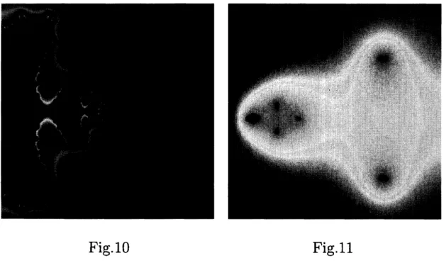
try to

Fig.

10

Fig.11

The unstable

manifold

of $P$, and the stable

manifold of

$Q$

are

shown in the

above.

Fig.12

In this

case

$(c=-0.7, b=0.3)$, in Fig.10, which represents

a

square region in the domain of definition of the Poincar\’e $s$ function, the pinched points

in the real axis

are

the points

on

the stable manifold of the other saddle point Q. Fig.11 shows the stable manifold of Q. The points in the real axis

of this Cantor-like set contains the intersection points with the unstable manifold, i.e. heteroclinic points.

In Fig.12, these two

curves

are

viewed.

Observe

tat the stable manifold of $Q$ intersects at the pinched point of the unstable manifold of P. As

these

curves

are in $\mathbb{C}^{2}$, they appear to intersect along a real curve, the

intersection is (numerically) transversal.

Fig.13 Fig.14

Fig.13 shows the unstable manifold of $Q$, and Fig.14 shows

an

enlargement

of right upper part. The unstable manifold picture in the domain of

defini-tion ofthe Poincar\’e‘s _{function is} similar to itself with respect to the origin

by the multiplication by the eigenvalue. However, small portion of it is not

necessarily similar to the whole picture. Note that this picture is

differ-ent from that ofthe unstable manifold of $P$, although further enlargement

reveals

some

detail similar to that of $P$, and vise-versa.

In Fig.15, the unstable manifold and the stable manifold of $Q$

are

plotted.

they intersect at pinching point of the Julia set in the unstable manifold. The intersection point in Fig.10 is away from the real axis. These in-tersection points

are

homoclinic points. NumericalIy, the intersection is transversal. Therefore, there must be

a

horseshoe. The invariant set in the

horseshoe is hidden in the Julia set and hard to recognize the Cantor set structure.

Fig.15

Fig.16 Fig17

Fig.16 and Fig.17 shows pictures with small portion of unstable manifold of $Q$ and the stable manifold of Q.

Although objects living in $\mathbb{C}^{2}$

are

quite hard to understand,

we can

try

to visualize them with the help of computer graphics. The color version of this note will be uploaded

on

the author’s web page:

http: $//www$

.

_math. $h$

.

kyoto-u.

ac.

jp$/\sim ushiki/$index. html

with interactive graphics software. Followings

are some

interesting pic-tures.

Fig.18

In this picture, the stable manifold of $Q$ (which is located at

a

pinched

location of the JUlia set) intersects with the unstable manifold of $P$ in two

points. The intersection is close to a heheroclinic tangency.

Fig.19

This picture shows

a

near-parabolic situation. Spiraling fixed points and

Fig.20

For

some

parameter, there is

a

case

with rabbit-like Julia set.

Some

part of the stable and unstable manifolds of $Q$ intersect in $Q($ the alpha fixed

point of the rabbit).

Fig.21 Fig.22

Fig.21 shows

a

part of the unstable manifold of $P$, and Fig.22 shows

a

part

of the unstable manifold of Q. They

are

embedded in $\mathbb{C}^{2}$

as

in the following

References

[1] E. Bedford, M.Lyubich, and J.Smilie, Distribution of periodic points of

polynomial diffeomorphisms of $\mathbb{C}^{2}$, Invent. Math. 114 (1993),

277-288.

[2] O.Biham, W.Wenzel: Unstable periodic orbits and the symbolic dy-namics of the complex H\’enon map, Phys. Rev. A42(1990),

4639-4646.

[3] J.H.Hubbard, The H\’enon _{mapping in the} complex domain, Chaotic dynamics and fractals (Atlanta, Ga.,1985), Academic Press, Orlando, FL,

1986, 101-111.

[4] H. Poincar\’e : Sur

une

classe nouvelle des transcendantes uniformes,