QUASI-ALTERNATING LINKS AND POLYNOMIAL INVARIANTS (Topology and Analysis of Discrete Groups and Hyperbolic Spaces)

全文

(1)33. 数理解析研究所講究録第2062巻 2018年 33-45. QUASI‐ALTERNATING LINKS AND POLYNOMIAL INVARIANTS MASAKAZU TERAGAITO. ABSTRACT. In this note, we survey several criteria for knots and links to be quasi‐alternating by using polynomial invariants such as Q ‐polynomials and Kauffman polynomials. Also, we mention two new generalizations of quasi‐alternating links.. 1. INTRODUCTION. Alternating knots and links give a classical but remarkable class of knots and links. The definition is described through diagrams, but it is very recent that a characterization without involving diagrams was. found by Greene [8] and Howie [12] independently.. On the other hand, there are a lot of generalizations of alternating knots and links in knot theory. Here is a list of adjectives, which is not complete. \bullet \bullet \bullet. \bullet \bullet \bullet. \bullet. \bullet \bullet. almost alternating, m‐almost alternating (Adams et al. [1]) toroidally alternating (Adams [2]) adequate (Lickorish‐Thistlethwaite [17]) semi‐alternating (Lickorish‐Thistlethwaite [17]) alternative (Kauffman [14]) pseudo‐alternating (Mayland‐Murasugi [19]) n‐semi‐alternating (Beltrami [3]) algebraically alternating (Ozawa [20]) quasi‐alternating (Ozsváth‐Szabó [21]). The objects of this note are quasi‐alternating knots and links intro‐ duced by Ozsváth and Szabó in their Heegaard Floer homology theory. Qua\mathcal{S}i ‐alternating links (abbreviated as QA links) are defined recur‐ sively as follows.. (1) The unknot is QA. 2010 Mathematics Subject Classification. Primary 57\mathrm{M}25, 57\mathrm{M}27. Key words and phrases. quasi‐alternating link, Q‐polynomial, Kauffman polynomial. The author has been partially supported by JSPS KAKENHI Grant Number \mathrm{J}\mathrm{P}16\mathrm{K}05149..

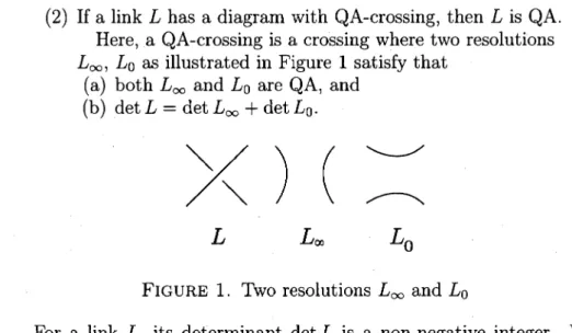
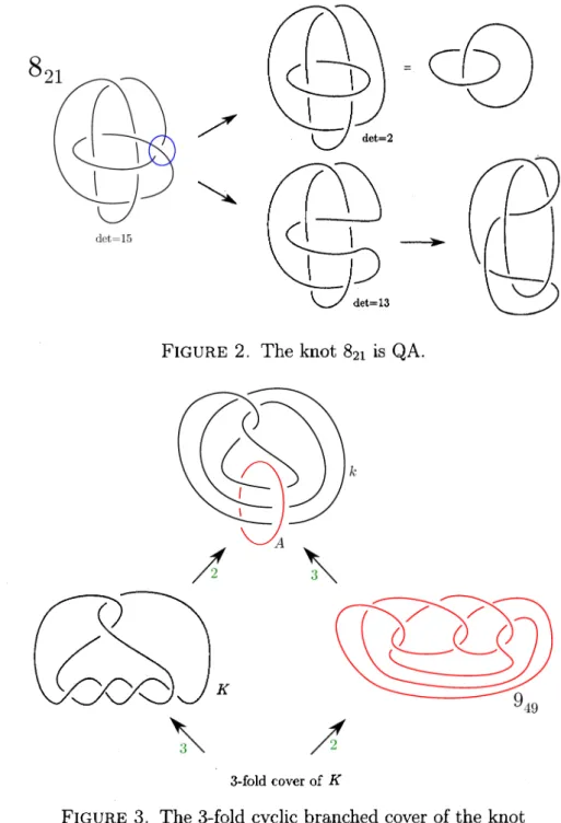
(2) 34 MASAKAZU TERAGAITO. (2) If a link. L. has a diagram with QA‐crossing, then. L. is QA.. Here, a QA‐crossing is a crossing where two resolutions. L_{\infty}, L_{0} as illustrated in Figure 1 satisfy that (a) both L_{\infty} and L_{0} are QA, and (b) \det L=\det L_{\infty}+\det L_{0}.. ) ( \wedge\ve L L_{\infty} L_{0} FIGURE 1. Two resolutions L_{\infty} and L_{0}. For a link L , its determinant \det L is a non‐negative integer. We should remark that if a link L is QA, then \det L>0 . Also, Ozsváth‐. Szabó [21] showed that any alternating knot and non‐split alternating. link are QA. Because of its recursive definition, it is not easy to identify whether a given knot or link is QA or not.. Problem 1.1. Decide whether a given knot or link is QA or not.. Example 1.2. The knot 8_{21} is non‐alternating, but QA. As illustrated in Figure 2, the marked crossing in the first diagram is a QA‐crossing. For, each of two resolutions is alternating, so QA, and we have the desired equality among their determinants. There are several properties of QA links: \bullet The double branched cover is an L‐space. \bullet The double branched cover bounds a negative‐definite 4‐manifold. H_{1}(W)=0. Homologically thin (knot Floer, reduced Khovanov, and re‐ W with. \bullet. duced odd Khovanov homologies are thin, i.e. supported on a. single diagonal.) Here is a digression. Let K be the (-2) ‐twist knot, which is the knot 5_{2} in the knot table. See Figure 3. Since K is 2‐bridge, its double branched cover is a lens space, which is a typical L‐space as its name suggests. Then, how about the 3‐fold cyclic branched cover? A direct approach is to calculate its Heegaard. Floer homology. As far as we know, there are some references [9, 16]. concerning Heegaard Floer homology of cyclic branched covers. Al‐ though we do not deny this approach, it would be hard to execute..

(3) 35 QUASI‐ALTERNATING LINKS AND POLYNOMIAL INVARIANTS. 8_{2^{1} \nearrow \searrow \det=15. FIGURE 2. The knot 8_{21} is QA.. \nearrow^{2} \nwarrow^{3}. sv. \nwarrow^{3} \nearrow^{2} 3‐fold cover of K. FIGURE 3. The 3‐fold cyclic branched cover of the knot 5_{2} is an L‐space.. However, there is a detour. Since K is 2‐bridge, it admits a cyclic pe‐ riod of order two. The image of K under this cyclic action is denoted by k in Figure 3. There, A is the image of the axis. We can see that.

(4) 36 MASAKAZU TERAGAITO. the factor knot k is unknotted. Hence the 3‐fold cyclic branched cover of k remains to be the 3‐sphere, and the lift of A gives the knot 9_{49}. Thus, the 3‐fold cyclic \mathrm{b}\mathrm{r}\mathrm{a}\mathrm{n}\mathrm{c}\mathrm{h}\mathrm{e}\mathrm{d}^{\backslash} cover of the original knot K is home‐ omorphic to the double branched cover of 9_{49} . In fact, 9_{49} is QA, so its double branched cover is an L ‐space. By the same technique, the 4‐ and 5‐fold cyclic branched covers of K are shown to be L‐spaces. without any calculation of Heegaard Floer homology [26, 11]. 2. CRITERIA BY Q ‐POLYNOMIAL. As mentioned before, it is not easy to determine whether a given knot. or link is QA or not, in general. However, Qazaqzeh and Chbili [22] found a very simple criterion for QA links in terms of Q ‐polynomials.. Theorem 2.1 ([22]). If a link. L. is QA_{f} then. \deg Q_{L}\leq\det L-1,. where \deg QL is the maximal degree of the Q ‐polynomial QL of L.. We recall the definition of Q ‐polynomials [4, 10]. Let L be an un‐ oriented link. Then its Q ‐polynomial Q_{L}(x) is a Laurent polynomial satisfying the following. (1) Q_{U}=1 , where U is the unknot. (2) Q_{L_{+}} +Q_{L_{-}} x(Q_{L_{\infty}} +Q_{L_{0}}) holds for the skein quadruple (L_{+}, L_{-}, L_{\infty}, L_{0}) as illustrated in Figure 4. =. ) ( L_{+} L_{-} L_{\infty} L_{0} FIGURE 4. The skein quadruple. For knots, their Q ‐polynomials have no negative powers of. Example 2.2. Let. fact,. K. Hence. K. be the knot 8_{19} , which is non‐alternating. In. is the (3, 4)‐torus knot. Then \deg Q_{K}. K. x.. =. 7. is not QA by Theorem 2.1.. and. \det K. =. 3.. The key of the argument of Qazaqzeh and Chbili [22] is the next. observation.. Lemma 2.3. Let L be a linkf and let L_{0} and L_{\infty} be two resolutions at some crossing of a diagram of L. Then. \displaystyle \deg Q_{L}\leq\max\{\deg Q_{L_{0}}, \deg Q_{L_{\infty}}\}+1..

(5) 37 QUASI‐ALTERNATING LINKS AND POLYNOMIAL INVARIANTS. Proof of Theorem 2.1. It is an induction on determinant. Let L be a 1 , so the 1 , then L is the unknot. Hence Q_{L} QA link. If dèt L inequality \deg Q_{L}\leq\det L-1 holds. Suppose \det L > 1 . Let L_{0} and L_{\infty} be two resolutions at a QA‐ crossing of L . Thus these are QA, and \det L_{*}<\det L\mathrm{f}\mathrm{o}\mathrm{r}*\in\{0, \infty\}. =. =. By Lemma 2.3,. \deg QL. \displaystyle \max\{\deg Q_{L_{0}}, \deg Q_{L_{\infty}}\}+1 < \displaystyle \max\{\det L_{0}, \det L_{\infty}\}+1 \leq. \leq \det L_{0}+\det L_{\infty}=\det L. \square. In [24], we gave an improvement of the criterion (Theorem 2.1) of. Qazaqzeh and Chbili.. Theorem 2.4 ([24]). If a link L is QA_{f} then one of the following holds. (1) L is a(2, n) ‐torus link (n\neq 0) and \deg Q_{L}=\det L-1 ; or (2) \deg Q_{L}\leq\det L-2. Example 2.5. Here are two examples which show that the evaluation. of Theorem 2.4(2) is optimal. (1) Let K be the figure‐eight knot. It is alternating, so QA, and \deg Q_{K}=3, \det K=5.. (2) Let. L. be the connected sum of two Hopf links. Since. split alternating, it is QA. And \deg Q_{L}=2,. L. \det L=4.. is non‐. Example 2.6. Each of non‐alternating knots 12_{n0025}, 12_{n0093}, 12_{n0115}, 11 . None of 12_{n0138} , 12_{n0199} , 12_{n0355}, 12_{n0374} has \deg Q 10, \det =. =. these is QA by our criterion (Theorem 2.4). This cannot be deduced by Theorem 2.1.. Here is a brief sketch of the proof of Theorem 2.4. The proof uses an induction on determinant. Let L be a non‐trivial QA link. Then the resolution at a QA crossing gives two QA links L_{\infty} and L_{0} . The argument is split into three cases.. (1) Neither L_{\infty} nor L_{0} is \mathrm{a}(2, n) ‐torus link. By the inductive hy‐ pothesis, \deg Q_{L_{*}} \leq\det L_{*}-2\mathrm{f}\mathrm{o}\mathrm{r}*\in\{\infty, 0\} . Then, \deg QL. \displaystyle \max\{\deg Q_{L_{\infty}}, \deg Q_{L_{0}}\}+1 = \deg Q_{L_{ $\alpha$}}+1 (\{ $\alpha$, $\beta$\}=\{\infty, 0\}) \leq (\det L_{ $\alpha$}-2)+1 = (\det L-\det L_{ $\beta$})-1 \leq. \leq \det L-2..

(6) 38 MASAKAZU TERAGAITO. (2) The case where one of L_{\infty}, L_{0} is \mathrm{a}(2, n)‐torus link is also easy. (3) If both are (2, *) ‐torus links, then we need another argument involving Dehn surgery. See [24]. 3. CRITERIA BY KAUFFMAN POLYNOMIAL. The previous argument in Section 2 works for Kauffman polynomial,. which is a two‐variable generalization of Q ‐polynomial [13]. Theorem 3.1. For a QA link. L,. either. (1) is a(2, n) ‐torus link (n\neq 0) , and \deg_{z}F_{L}=\det L-1 ; or (2) \deg_{z}F_{L}\leq\det L-2. L. For a diagram D of an oriented link L, $\Lambda$_{D}(a, z) is defined with forgetting its orientation as follows:. (1) $\Lambda$_{D} is a regular isotopy invariant; (2) For the unknot diagram without crossing U, $\Lambda$_{U}=1 ; (3) $\Lambda$_{L+}+$\Lambda$_{L_{-} =z($\Lambda$_{L_{\infty} +$\Lambda$_{L_{0} ) ; (4) If. D. $\Lambda$_{6}\backslash =a^{-1}$\Lambda$_{\mathrm{v}. $\Lambda$_{\mathrm{b}^{-} =a$\Lambda$_{\vee} has writhe. w. , then the Kauffman polynomial of. F_{L}(a, z)=a^{-w}$\Lambda$_{D}(a, z). L. is defined as. .. Since F_{L}(1, z)=Q_{L}(z) , we have \deg Q_{L}\leq\deg_{z}F_{L} , where \deg_{z}F_{L} is the maximal degree of variable z.. For alternating ones among QA links, a classical fact by R. Crowell. [6] implies the following.. Theorem 3.2. For a non‐split alternating link. (1) (2). L L. L,. either. is a(2, n) ‐torus link (n\neq 0) , and \deg_{z}F_{L}=\det L-1 ; is the figure‐eight knot or Hopf link \# Hopf link, and \deg_{z}F_{L}=. \det L-2 ; or. (3) \deg_{z}F_{L}\leq\det L-3. For non‐alternating QA links, we have the following.. Theorem 3.3 ([25]). For non‐alternating QA link L , either (1) d\mathrm{e}\mathrm{g}_{z}F_{L}\leq\det L-3 ; or (2) L has exactly 3 components, each of which is unknotted. More‐ over,. L. is obtained from the Hopf link by a banding on one. component.. We expect that the second possibility of Theorem 3.3 would not hap‐ pen, but we could not erase it. As an immediate corollary of Theorem 3.3, we have the following criterion for non‐alternating QA knots..

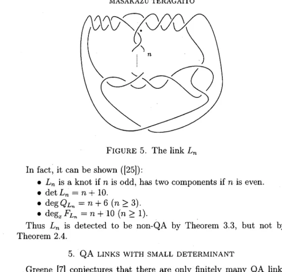
(7) 39 QUASI‐ALTERNATING LINKS AND POLyNOMIAL INVARIANTS. Corollary 3.4. For a non‐alternating QA knot K_{\mathrm{Z} we have. \deg Q_{K}\leq\deg_{z}F_{K}\leq\det K-3. Example 3.5. The evaluation of Corollary 3.4 is sharp. Let K be the (-3,2, n) ‐pretzel knot, n \geq 3 odd. This knot has the following properties. \bullet. K. is non‐alternating QA.. \bullet. \det K=n+6.. \bullet. \deg Q_{K}=\deg_{z}F_{K}=n+3.. Example 3.6. Let K=9_{46} , which is the (-3,3,3) ‐pretzel knot. Then. it satisfies: \bullet. \bullet. K. is non‐alternating.. \det K=9.. \deg Q_{K}=\deg_{z}F_{K}=7. Hence, K is not QA by Corollary 3.4. This fact was known by its thick \bullet. Khovanov homology (see [5, page 2456 Finally, we propose a problem on the a‐span, denoted by \mathrm{s}\mathrm{p}\mathrm{a}\mathrm{n}_{a}F_{L}, of the Kauffman polynomial F_{L}(a, z) for QA link L . If L is non‐split alternating, then \mathrm{s}\mathrm{p}\mathrm{a}\mathrm{n}_{a}F_{L} is equal to its crossing number by [27]. Hence the inequality \mathrm{s}\mathrm{p}\mathrm{a}\mathrm{n}_{a}F_{L}\leq\det L holds. We expect that this would hold for QA links. Problem 3.7. Let L be a. QA. link.. (1) Show that \mathrm{s}\mathrm{p}\mathrm{a}\mathrm{n}_{a}F_{L}\leq\det L. (2) Show that \mathrm{s}\mathrm{p}\mathrm{a}\mathrm{n}_{a}F_{L} \leq span V_{L} polynomial of L.. \leq \det L_{f}. where V_{L} is the Jones. These are verified for all QA knots up to 11 crossings. The second inequality \mathrm{s}\mathrm{p}\mathrm{a}\mathrm{n}V_{L}\leq\det L of Problem 3.7(2) is mentioned in [22]. 4. Q ‐POLYNOMIAL VERSUS KAUFFMAN POLYNOMIAL. It is possible that \deg Q_{L}<\deg_{z}F_{L} . Hence there is a chance that the. criterion (Theorem 3.3) by the Kauffman polynomial is strictly stronger than one (Theorem 2.4) by the Q‐polynomial. The next shows that it can happen.. Theorem 4.1. There exist infinitely many hyperbolic knots and links L_{n} such that. (1) L_{n} is not QA ; (2) \deg Q_{L_{r $\iota$}}=\det L_{n}-4 ; and (3) \deg_{z}F_{L_{n}}=\det L_{n}..

(8) 40 MASAKAZU TERAGAITO. FIGURE 5. The link L_{n}. In fact, it can be shown ([25]): \bullet. \bullet \bullet \bullet. L_{n} is a knot if n is odd, has two components if \det L_{n}=n+10.. \deg Q_{L_{ $\tau \iota$}}=n+6(n\geq 3) \deg_{z}F_{L_{n}}=n+10(n\geq 1). n. is even.. .. .. Thus L_{n} is detected to be non‐QA by Theorem 3.3, but not by Theorem 2.4.. 5. QA LINKS WITH SMALL DETERMINANT. Greene [7] conjectures that there are only finitely many QA links. with a given determinant. He determined all QA knots and links with determinant \leq 3 as shown in Table 1.. TABLE 1. QA links with determinant \leq 3. We proved in [24, 25] the followings. Theorem 5.1. If L is a QA link with \det L=4 , then L is the (2, \pm 4)torus link_{J} or L has 3 components, each of which is unknotted, and \deg_{z}F_{L}\leq 2.. Theorem 5.2. If L is a QA link with \det L=5_{f} then figure‐eight knot or the (2, \pm 5) ‐torus knot.. L. is either the.

(9) 41 QUASI‐ALTERNATING LINKS AND POLYNOMIAL INVARIANTS. After that, Lidman and Sivek [18] classified all QA links with \det\leq 7. based on the determination of all formal. L‐spaces. with order at most. 7.. Theorem 5.3 ([18]). QA links with \det\leq 7 are 2‐bridge or a connected sum of 2‐bndge links.. Thus all QA links with \det\leq 7 are determined as in Table 2.. TABLE 2. QA links with determinant. \leq 7. Problem 5.4. (1) Solve Greenefs conjecture. (2) Determine QA links with \det=8. We remark that the pretzel link P(-3,2,2) is non‐alternating QA. and \det=8.. 6. WEAKLY QUASI‐ALTERNATING LINKS. In the remaining two sections, we mention two recent generalizations of QA links. The first one is weakly quasi‐alternating links introduced. by D. Kriz and I. Kriz [15]. Weakly quasi‐alternating links (abbreviated as WQA links) are de‐ fined recursively as follows.. (1) The unknot and unlinks are WQA. (2) If a link L has a diagram with WQA‐crossing, then. L. is WQA.. Here, a WQA‐crossing is a crossing where two resolutions L_{\infty}, L_{0} satisfy. (a) both L_{\infty} and L_{0} are WQA, and (b) \det L=\det L_{\infty}+\det L_{0}. For a split link, its determinant is 0 . Hence, any split link is WQA. Thus we think that this class would be too wide.. Kriz‐Kriz [15] showed: Theorem 6.1 ([15]).. (1) Any WQA link is BOS thin..

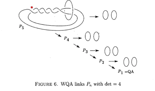
(10) 42 MASAKAZU TERAGAITO. (2) The double branched cover of a WQA knot. i\mathcal{S}. an. L ‐space.. Baldwin‐Ozsváth‐Szabó cohomology H_{BOS} is an invariant of oriented links. A link L is BOS thin if rank. H_{BOS}^{i}(L)=. \left{\begin{ar y}{l \detL,&\mathr{i}\mathr{f}i=$\sgma$(L)/2,\ 0,&\mathr{o}\mathr{}\mathr{}\mathr{e}\mathr{}\mathr{w}\mathr{i}\mathr{s}\mathr{e}. \nd{ar y}\ight.. For QA links, Greene conjectures that there are only finitely many QA links with a given determinant, but the same thing does not hold for WQA links. Theorem 6.2. Let d\geq 0 be a multiple of 4 or a square (> 1) . Then there exist infinitely many WQA, non‐QA links with \det=d.. Example 6.3. The (-2,2, n) ‐pretzel link P_{n} has \det=4 for any inte‐ ger n . For example, P_{0} is Hopf link \# Hopf link, P_{1} is the (2, 4)‐torus link. Also, \deg Q_{P_{n}}=|n|+2 . Hence P_{n} is \mathrm{n} ot QA if |n| \geq 2 , but P_{n} is WQA as illustrated in Figure 6.. \rightarrow 00. \searrow_{P_{4}}\rightarrow 00. \searowP_{3}\searow_{P 2_{\searow_{P 1}=\mathrm{Q}\mathrm{A}^{\rightarow}\rightarow0_{0}. FIGURE 6. WQA links P_{n} with. \det=4. Although we do not give the proof of Theorem 6.2, the pretzel link P(-l, l, m) (3 \leq l \leq m) gives an example for a square determinant. Let L=P(-l, l, m) . Then \det L=l^{2} , and any crossing in the m‐twist strand is WQA. By [7], L is not QA. Also, any Kanenobu knot is shown to be WQA. They have determi‐ nant 25, and it is known that there are only finitely many QA Kanenobu. knots (22). Question 6.4. Let \det=d^{l}?. 1 \leq d \leq 3 .. Is there a WQA, non‐QA link with.

(11) 43 QUASI‐ALTERNATING LINKS AND POLYNOMIAL INVARIANTS. 7. TWO‐FOLD QUASI‐ALTERNATING LINKS. Scaduto and Stoffregen [23] introduced two‐fold quasi‐alternating links. We will not give full details (see [23]). For a link, a marking assigns 0 or 1 to each component of L . The weight 1 is expressed as one dot on the čomponent. The total number of dots is required to be even. After a resolution, the dots are carried in the natural way. w. Two‐fold quasi‐alternating links (abbreviated as TQA links) are de‐ fined recursively as follows.. (1) The unknot with trivial marking is TQA. (2) A split union of two odd‐marked links is TQA. (3) L is TQA if it has TQA crossing where two resolutions L_{\infty} and L_{0} satisfy. (a) both of L_{\infty} and L_{0} are TQA, (b) \det L=\det L_{\infty}+\det L_{0}. It is not hard to see that \mathrm{Q}\mathrm{A}\Rightar ow \mathrm{T}\mathrm{Q}\mathrm{A}\Rightar ow \mathrm{W}\mathrm{Q}\mathrm{A} , in general. As a typical example, Figure 7 shows that the non‐QA knot 11_{n50} is TQA. (Dots on the same component is counted \mathrm{m}\mathrm{o}\mathrm{d} 2. ). FIGURE 7. The non‐QA. \mathrm{k}\mathrm{n}\mathrm{q},\mathrm{t}. It is shown in [23] that a TQA link is. 11_{n50} is TQA.. \mathrm{m}\mathrm{o}\mathrm{d} 2. Khovanov thin. Also,. the framed instanton homology of the double branched cover of a TQA link is examined there..

(12) 44 MASAKAZU TERAGAITO. REFERENCES. 1. C. Adams, J. Brock, J. Bugbee, T. Comar, K. Faigin, A. Huston, A. Joseph. and D. Pesikoff, Almost alternating links, Topology Appl. 46 (1992), no. 2, 151−165.. 2. C. Adams, Toroidally alternating knots and links, Topology 33 (1994), no. 2, 353‐369.. 3. E. Beltrami, Arc index of non‐alternating links, J. Knot Theory Ramifications. 11 (2002), no. 3, 431‐444.. 4. R. D. Brandt, W. B. R. Lickorish and K. C. Millett, A polynomial invariant. for unoriented knots and links, Invent. Math. 84 (1986), no. 3, 563‐573.. 5. A. Champanerkar and I. Kofman, Twisting quasi‐alternating links, Proc. Amer.. Math. Soc. 137 (2009), no. 7, 2451‐2458. 6. R. Crowell, Nonalternating links, Illinois J. Math. 3 (1959), 101‐120. 7. J. Greene, Homologically thinf non‐quasi‐alternating links, Math. Res. Lett. 17. (2010), no. 1, 39‐49. 8. J. Greene, Alternating links and definite surfaces, preprint, arXiv: 1511.06329. 9. J. Grigsby, Knot Floer homology in cyclic branched covers, Algebr. Geom.. Topol. 6 (2006), 1355‐1398. 10. C. F. Ho, A new polynomial for knots and links‐ preliminary report, Abstracts. Amer. Math. Soc. 6 (1985), no. 4, 300, Abstract 821‐57‐16. 11. M. Hori, On cyclic branched covers of knots and. L ‐space. conjecture, master. thesis (in Japanese), Hiroshima University. 12. J. Howie, A characterization of alternating knots, preprint, arXiv: 1511. 04945. 13. L. H. Kauffman, An invariant of regular isotopy, Trans. Amer. Math. Soc. 318. (1990), no. 2, 417−471.. 14. L. Kauffman, Combinatorics and knot theory, in Low‐dimensional topology. (San Francisco, Calif., 1981), 181‐200, Contemp. Math., 20, Amer. Math. Soc., Providence, RI, 1983.. 15. D. Kriz and I. Kriz, A spanning tree cohomology theory for links, Adv. Math.. 255 (2014), 414‐454.. 16. A. Levine, Computing knot Floer homology in cyclic branched covers, Algebr.. Geom. Topol. 8 (2008), no. 2, 1163‐1190.. 17. W. Lickorish and M. Thistlethwaite, Some links with nontntvial polynomials. and their crossing‐numbers, Comment. Math. Helv. 63 (1988), no. 4, 527‐539. 18. T. Lidman and S. Sivek, Quasi‐alternating links with small determinants, preprint, arXiv: 1507. 04705.. 19. E. Mayland and K. Murasugi, On a structural property of the groups of alter‐. nating links, Canad. J. Math. 28 (1976), no. 3, 568‐588. 20. M. Ozawa, Rational structure on algebraic tangles and closed incompressible surfaces in the complements of algebraically alternating knots and links, Topol‐. ogy Appl. 157 (2010), no. 12, 1937‐1948.. 21. P. Ozsváth and Z. Szabó, On the Heegaard Floer homology of branched double‐. covers, Adv. Math. 194 (1) (2005), 1‐33.. 22. K. Qazaqzeh and N. Chbili, A new obstruction of quasi‐alternating links, Al‐. gebr. Geom. Topol. 15 (2015), 1847‐1862. 23. C. Scaduto and M. Stoffregen, Two‐fold quasi‐alternating links, Khovanov ho‐ mology and instanton homology, preprint, “Xiv: 1605. 05394..

(13) 45 QUASI‐ALTERNATING LINKS AND POLYNOMIAL INVARIANTS. 24. M. Teragaito, Quasi‐alternating links and Q\rightar owpolynomials, J. Knot Theory Ram‐ ifications 23 (2014), no. 12, 1450068, 6 pp. 25. M. Teragaito, Quasi‐alternating links and Kauffman polynomials, J. Knot The‐ ory Ramifications 24 (2015), no. 7, 1550038, 17 pp. 26. M. Teragaito, Fourfold cyclic branched covers of genus one two‐bridge knots are L ‐spaces,. Bol. Soc. Mat. Mex. (3) 20 (2014), no. 2, 391‐403.. 27. Y. Yokota, The Kauffman polynomial of alternating links, Topology Appl. 65. (1995), no. 3, 229‐236. DEPARTMENT OF MATHEMATICS AND MATHEMATICS EDUCATION, HIROSHIMA UNIVERSITY, 1‐1‐1 KAGAMIYAMA, HiGASHi−HiROSHiMA 739-8524 , JAPAN E‐mail address: teragai@hiroshima‐u.ac.jp.

(14)