Origin of RHEED Intensity Oscillation during
Homoepitaxial Growth on Si(001)
T. Kawamura1 and P. A. Maksym2
1 Department of Mathematics and Physics, University of Yamanashi, Kofu, Yamanashi
400-8510, Japan
2Department of Physics and Astronomy, University of Leicester, University Road,
Leicester, LE1 7RH, UK
Abstract
The origin of RHEED intensity oscillations or variations during growth is analysed by using RHEED intensity distributions calculated from wave func-tions inside and outside the crystal surface. When the growth proceeds in a layer by layer fashion and the observed intensity is near a diffraction peak, there are only two possible origins of the intensity variations. One is the interference between waves diffracted by the top and the subsequent under-lying layers, and the other is the disturbance of the RHEED electron waves by step edges. RHEED rocking curves are computed and the intensities of peaks in the curves are found to vary systematically when material is de-posited on the surface. The mechanism of these variations is identified by computing RHEED intensity distributions. An approximate measure of the disturbance of the wave function by step edges is also introduced.
Keywords: Electron-solid diffraction, RHEED intensity oscillation, wave function, MBE growth, step density, Si(001)
1. Introduction
Since the first observation of oscillations in the intensity of reflection high energy electron diffraction (RHEED) during growth by molecular beam epitaxy [1], RHEED has become widely used for monitoring and controlling the growth. This is mainly because the period of the specular beam intensity oscillation of RHEED corresponds to growth of a monolayer or bilayer of film on the substrate crystal (assuming a layer-by-layer growth mode). The origin
of the RHEED intensity oscillation has been widely studied [1, 2, 3, 4, 5, 6, 7] but is still not fully understood. One possible origin is interference between waves diffracted from two layers with a monolayer height difference at an off-Bragg condition [2]. Another possible origin is diffuse scattering due to roughness of the surface. This comes from the idea of similarity to the diffuse scattering of light because the reflectivity of light from a surface decreases as its roughness increases [1]. Yet another possible origin is changes in the surface step density because the roughness increases as step density increases [8]. Finally, a slightly different possible cause of the oscillations is a change in the in-plane lattice spacing as occurs during homoepitaxial growth on AlSb [7].
Recently, the origin of the oscillations has been studied by calculating the RHEED wave function [9, 10] with multiple scattering theory [11, 12]. In the case of homoepitaxial growth on Si(001) with an incident energy of 30 keV and glancing angle around 1◦, the period of the intensity oscillation corresponds to a monolayer and the origin of the oscillation is the interference between waves scattered by two successive layers with a monolayer height difference [11]. In the case of homoepitaxial growth on GaAs(001) with an incident energy of 15 keV and glancing angle around 1◦, the period of the
intensity oscillation corresponds to a monolayer of Ga and As, i.e., two layers, and the origin is the scattering at step edges toward non-specular directions [12].
In this paper, we will study the origin of RHEED intensity oscillation from surfaces with steps of atomic monolayer and bilayer height in order to elucidate a unified view of the origin in the case of homoepitaxial growth on Si(001). For modeling the growth in a layer-by-layer fashion, we use 16× 1 and 1× 16 supercells of the Si(001) with steps of either monolayer or bilayer height and ignore surface reconstruction. We choose typical incident beam conditions: an energy of 15 keV, glancing angles between 1◦ and 4◦ with the
incident beam azimuth in the [110] direction, either perpendicular to or par-allel to the dangling bond direction of the top Si atom. We calculate specular beam intensities and wave functions from the stepped Si(001) surfaces with a multiple scattering theory [13, 14].
2. Calculation
As a crystal surface has two dimensional periodicity, the wave function has the form of a two-dimensional Bloch wave and can be written as
Ψ(r) = exp(i k∥· ρ)!
κ φκ(z ) exp(iκ · ρ).
(1) Here κ is a two-dimensional reciprocal lattice vector, k∥is the surface parallel component of the incident electron wave vector k and ρ, z are the parallel and normal components of the position vector r. The z-axis is taken to be normal to the surface with the positive direction from the surface to vacuum. The reflected intensities are calculated by solving the Schr¨odinger equation for the wave function
∇2Ψ(r) + k2Ψ(r) = 2m
!2 V (r)Ψ(r) (2)
according to the algorithm of Maksym and Beeby [13, 14].
To analyse the RHEED intensity oscillations, we use the absolute square of the wave function,
I(k, r) =|Ψk(r)|2. (3)
We call this the electron intensity (EI) and it is a function of 3 dimensions in space. It is not easy to plot the 3-dimensional EI on a sheet of paper so to visualise it we use the cross sectional EI (CSEI). The CSEI is defined for a fixed y value, y0, as I(k,x,y0,z). As y is taken to be along the incident
beam azimuth, the variation of the EI as a function of y is small. We have calculated CSEIs by changing y and confirmed the small variation along y [10]. We hereafter ignore the y dependence and write I(k,x,y0,z) as I(k,x,z).
In the following calculations, we put y0=0.5a. Here the unit length of the
Si(001) surface is denoted as a=a0/
√
2 with a0 the lattice constant of a Si
crystal. The details of the calculation of the wave function and CSEI are given in a previous paper [10]. We also use the CSEI averaged over the x direction, which is defined by
Iav(k, z) = 1 l " l 0 I(k, x, z)dx. (4)
Here l is a unit length of the lattice in the x-direction and l is 16a for a 16×1 supercell and a for a 1× 16 supercell or a 1 × 1 cell in the present paper.
3. Specular beam rocking curves
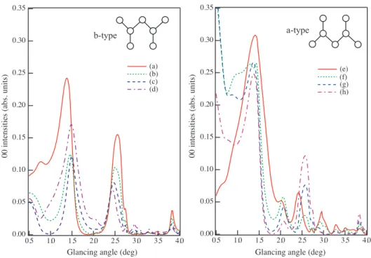
The calculated rocking curves of the specular beam are shown in Fig. 1. In the calculation 23 beams (9 beams in the zeroth Laue zone and 7 beams in the first and minus first Laue zones) are taken into account. The flat Si(001) surface can have two different structures, depending on which atomic plane is at the surface. In one structure (the a-type surface) the dangling bond direction of the topmost atom is normal to [110] and in the other (the b-type surface) it is parallel to [110] as depicted in the insets. The two panels of Fig. 1 show how the intensity changes during a growth cycle in which 2 monolayers are deposited on the b-type surface. The left hand panel shows the rocking curve for the flat b-type surface and curves for a-type islands deposited on the b-type surface. The right hand panel shows the rocking curve for the flat a-type surface that occurs after deposition of one monolayer and curves for b-type islands deposited on the a-type surface. The bilayer growth cycle in the supercell actually results in 32 rocking curves but for clarity only eight curves are shown in the figure.
The rocking curve from the b-type flat surface is curve (a). Curves (b), (c) and (d) are those from surfaces with an island of monoatomic height consisting of 4, 8 and 12 atomic rows, respectively of the a-type surface running parallel to the beam azimuth. Curve (e) is that from the a-type flat surface. Curves (f), (g) and (h) are those from surfaces with an island consisting of 4, 8 and 12 atomic rows of b-type surface, respectively running normal to the beam azimuth. It has been reported that islands are likely to grow anisotropically with their longer dimension normal to the dangling bond direction [15]. Therefore the islands in the calculation of curves (f), (g) and (h) are elongated along the direction normal to the incident beam azimuth and the intensities are calculated by using a 1× 16 supercell rather than a 16× 1 supercell.
The specular beam intensities from the b-type surface show three major peaks at 1.38◦, 2.56◦ and 3.84◦ and those from the a-type surface show five
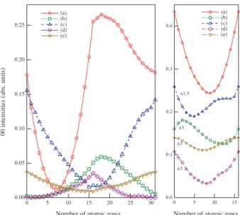
major peaks at 1.40◦, 2.02◦, 2.42◦, 2.96◦ and 3.28◦ in the angle range between 0.5◦ and 4.0◦. The left panel of Fig. 2 shows the intensity as a function of the number of atomic rows when the glancing angle is 1.22◦, 2.04◦, 2.56◦,
2.96◦ and 3.84◦. The intensity clearly varies systematically. For example, at 1.22◦ the intensity decreases to below that from the b-type surface as the number of atomic rows increases from 1 to 7 and then increases as the number of atomic rows increases from 8 to 18. It is near its maximum when
0.35 0.30 0.25 0.20 0.15 0.10 0.05 0.00
00 intensities (abs. units)
4. 0 3. 5 3. 0 2. 5 2. 0 1. 5 1. 0 0. 5
Glancing angle (deg) (e) (g) (h) 0.35 0.30 0.25 0.20 0.15 0.10 0.05 0.00 4. 0 3. 5 3. 0 2. 5 2. 0 1. 5 1. 0 0. 5 (a) (b) (c) (d) 00 intens iti es (a bs. un its)
Glancing angle (deg)
(f)
b-type a-type
Figure 1: Left: Specular beam rocking curves from a flat b-type surface (a), from 16× 1
supercell surfaces with one a-type island of monolayer height with 4 (b), 8 (c) and 12 (d) atomic rows on top of the b-type surface. Right: Specular beam rocking curves from a flat a-type surface (e), from 1×16 supercell surfaces with one b-type island of monolayer height with 4 (f), 8 (g) and 12 (h) atomic rows on top of the a-type surface. The insets show the atomic arrangement of the top three atomic layers projected onto a plane perpendicular to the [110] direction (schematic).
0.25 0.20 0.15 0.10 0.05 0.00
00 intensities (abs. units)
30 25 20 15 10 5 0
Number of atomic rows
(a) (b) (c) (d) (e) 0.4 0.3 0.2 0.1 0.0 15 10 5 0
Number of atomic rows
x1.5 x3 x3 x3 (a) (b) (c) (d) (e)
Figure 2: The specular beam intensities as a function of the number of atomic rows on b-type surface from 0 to 31 at the glancing angles of 1.22◦ (a), 2.04◦(b), 2.56◦ (c), 2.96◦ (d) and 3.84◦ (e). The left panel shows the intensities from a single domain surface. The right panel shows the intensities from surfaces with 2 domains calculated by assuming no interference between waves from different domains. The intensities are multiplied by 1.5 at the glancing angle of 2.04◦ and by 3 at the glancing angles of 2.56◦, 2.96◦ and 3.84◦.
the surface is of a-type and flat (e) and the exact maximum occurs when there are 2 b-type atomic rows on the a-type surface. Further increase in the number of atomic rows from 19 to 31 then results in decreasing intensity. When the glancing angle is 2.04◦ (b) and 2.96◦ (d) in Fig. 2, the specular
intensity shows a near maximum and exact maximum for the a-type flat surface, while it shows a near minimum and exact minimum for the b-type flat surface, respectively. When the glancing angle is 2.56◦ (c) and 3.84◦ (e),
the specular intensity shows a near minimum and exact minimum for the a-type flat surface, respectively, while it shows a maximum for the b-a-type flat surface. In other words, the behaviour at 2.56◦ and 3.84◦ is opposite to that
seen at 2.04◦ and 2.96◦. The period of the intensity variation at 1.22◦, 2.04◦,
2.56◦, 2.96◦ and 3.84◦corresponds to growth of a bilayer. We will discuss the
origin of these intensity oscillations in the following sections.
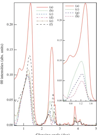
Fig. 3 shows a series of rocking curves from Si(001) surfaces with steps of bilayer height. The incident beam azimuth is parallel to the dangling bond direction of the topmost atoms, i.e. the surfaces are b-type. When the
glancing angle is 1.22◦, 2.56◦ and 3.84◦, the specular beam intensity varies
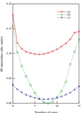
systematically as a function of the number of atomic rows on a surface as shown in Fig. 4.
At these glancing angles, the specular beam intensity shows a maximum for the flat surface and decreases when the number of atomic rows increases. A minimum occurs when the number of rows is 6, 8 and 7 at the glancing angles of 1.22◦, 2.56◦ and 3.84◦, respectively. In Figs. 3 and 4, the difference
in intensities from the stepped surface with 4, 6, 8 and 10 atomic rows is small at 1.22◦. The inset in Fig. 3 shows rocking curves for the case when the number of atomic rows is fixed at 6 but the number of steps, that is, the step density is changed. Curve (c) shows the rocking curve from a surface with one island of 6 atomic rows and this is the same as (c) in the main figure. Curves (g) and (h) show curves from 2 islands consisting of 3 atomic rows and from 3 islands consisting of 2 atomic rows, respectively. The intensity around 1.22◦ decreases as the step density increases.
4. Intensity variations at 1.22◦ 4.1. Surfaces with monolayer steps
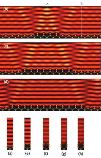
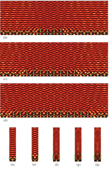
In order to analyse the origin of the intensity variation we calculate the CSEIs for the various numbers of atomic rows in Fig. 1. The results are shown in Fig. 5. Part (a) shows the CSEIs from a b-type flat surface calculated by using a 1×1 unit cell. (b), (c) and (d) show CSEIs from 16×1 surfaces with a single island consisting of 4, 8 and 12 a-type atomic rows on a b-type surface. (e) shows the CSEI from the a-type flat surface, (f), (g) and (h) show CSEIs from 1×16 surfaces with a single island consisting of 4, 8 and 12 b-type atomic rows on an a-type surface. The CSEIs show periodic variations of bright and dark contrast along the surface normal. The brighter contrast corresponds to the higher intensity. The positions of the maximum electron intensities above the topmost layer correspond to those of the minimum intensities above the second topmost layer and vice versa in Figs. 5 (b), (c) and (d). This CSEI variation is similar to the CSEI variations at the glancing angle of 0.98◦ for
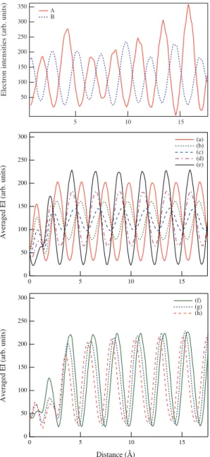
the energy of 30 keV reported previously [11]. The upper figure in Fig. 6 shows the CSEI variations I(k,x,z) as a function of the distance (z) along the lines A (x = 7.5a) and B (x = 13a) as indicated in Fig. 5 (b). The two curves show oscillatory variations with almost opposite phases. This phase difference results in the lowest EI when the number of atomic rows in the topmost layer is the same as that in the second layer.
0.20
0.15
0.10
0.05
0.00
00 intensities (abs. units)
5 4
3 2
1
Glancing angle (deg)
(a) (b) (c) (d) (e) (f) 0.20 0.15 0.10 0.05 0.00 1.6 1.2 0.8 (a) (c) (g) (h)
Figure 3: Specular beam rocking curves from 16× 1 supercell surfaces of various atomic
density in the topmost layer when the step density is fixed at 0.125. (a) flat b-type surface, surfaces with one island of bilayer height with (b) 4, (c) 6, (d) 8, (e) 10 and (f) 12 atomic rows on top of the b-type surface. The inset shows the rocking curves in the low glancing angle region. (a) and (c) are the same as in the main figure. (g) and (h) are the curves from surfaces with 4 steps (2 islands of 3-atomic rows) and 6 steps (3 islands of 2-atomic rows) with the total number of atomic rows fixed at 6.
0.20
0.15
0.10
0.05
0.00
00 intensities (abs. units)
15 10 5 0 Number of rows (a) (b) (c)
Figure 4: Specular beam intensities as a function of the number of atomic rows of bilayer height on the b-type surface at glancing angles of 1.22◦ (a), 2.56◦ (b) and 3.84◦ (c).
(a) (a) (b) (b) (c) (c) (d) (d) (e) (e) (f) (f) (g) (g) (h) (h) A B
Figure 5: CSEIs from 16× 1 supercell surfaces with (a) 0, (b) 4, (c) 8 and (d) 12 a-type
atomic rows on a b-type surface when the step density is fixed (0.125). CSEIs from 1× 16
supercell surfaces with (e) 0, (f) 4, (g) 8 and (h) 12 b-type atomic rows on an a-type
surface. The incident beam glancing angle is 1.22◦. The lines A, B show the lines along
which the intensity data is plotted in Fig. 6. The small circles indicate the atomic sites of the surface and the bonds between them are shown by the hexagonal network of lines. The dashed lines in (f), (g) and (h) indicate bonds between atoms in the top and the second layer when 4, 8 and 12 toptmost atomic sites are occupied, respectively.
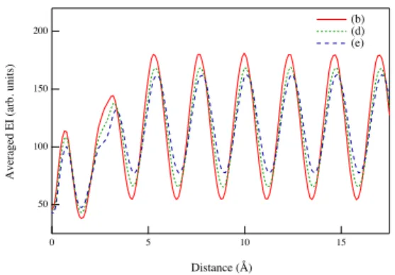
The center and lower panels of Fig. 6 show the intensity variations of Iav(k, z) (Eq. 4) in Fig. 5 as a function of position, z, from the surface (z=0
˚
A) to outside the crystal (z=17.5 ˚A). Except for the region around the top surface layer, each curve of Iav(k, z) shows an oscillation of approximately
constant amplitude. The amplitude has a near maximum for the a-type flat surface (e) and for a surface with 4 b-type atomic rows formed on an a-type surface (f). The amplitude decreases as the number of b-type atomic rows increases from 4 (f) to 16 (a) on the a-type surface. It further decreases as the number of a-type atomic rows increases on the b-type surface. It goes through a near minimum when the number of atomic rows is 8 (c) and one half of the surface is covered with the growing a-type layer. The variation of the oscillation amplitudes corresponds to the variation of the specular beam intensity shown in Figs. 1 and 2.
To obtain further insight into the scattering process, the variation of Iav(k, z) is compared with the weighted sum of the CSEIs above the a-type
surface and the b-type surface. The CSEIs above the a-type and b-type surfaces are denoted by Ia
av(k, z) and Iavb(k, z), respectively, and the weighted
sum is calculated as
Isum(σn, z) = σnIava (k, z) + (1− σn)Iavb(k, z). (5)
Here σn=n/16 is the atomic row density of the topmost layer. When the
disturbance of the standing waves from flat parts of the surface caused by steps is small, Iav(k, z) and Isum(σn, z) show excellent agreement. Then the
difference
∆Istep= Isum(σn, z)− Iav(k, z) (6)
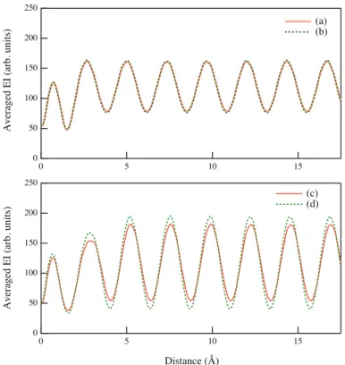
is a good measure of the disturbance caused by steps. The upper part of Fig. 7 shows an example of the comparison of Iav(k, z) and Isum(σn, z). In this
case n = 4 (solid curve) and Isum(σn, z) is calculated with σn=0.25 (dotted
curve). The two curves show excellent agreement. Similar agreement is found for n = 8 and n = 12 and this is consistent with the relatively small influence of the steps in Fig. 5.
4.2. Surfaces with bilayer steps
The intensity variations are analysed by calculating CSEIs corresponding to the rocking curves in Fig. 3. Fig. 8 shows CSEIs at 1.22◦ from 16× 1 surfaces. Parts (a) - (c) show CSEIs from surfaces with an island consisting of 4, 6 and 8 atomic rows of bilayer height on the b-type surface when the step
350 300 250 200 150 100 50 El ec tro n i nt en sit ies (a rb . u ni ts) 15 10 5 A B 300 250 200 150 100 50 0
Averaged EI (arb. units)
15 10 5 0 (a) (b) (c) (d) (e) 300 250 200 150 100 50 0
Averaged EI (arb. units)
15 10 5 0 Distance (Å) (f) (g) (h)
Figure 6: The upper panel shows CSEIs along the lines A and B in Fig. 5 (b). The center and lower panels show the intensity variations of Iav(k, z) in Fig. 5. Curves (a), (b), (c), (d), (e), (f), (g) and (h) correspond to the CSEIs (a), (b), (c), (d), (e), (f), (g) and (h) in Fig. 5, respectively.
250 200 150 100 50 0 Averaged EI (arb. units) 15 10 5 0 (a) (b) 250 200 150 100 50 0
Averaged EI (arb. units)
15 10 5 0 Distance (Å) (c) (d)
Figure 7: Comparison of Iav(k, z) with Isum(σn, z) at the glancing angle 1.22◦. In the
upper panel, curve (a) is Iav(k, z) obtained from Fig. 5 (b) and curve (b) is Isum(σn, z) calculated by using Eq. 5 with n=4 (b). In the lower panel, curve (c) is Iav(k, z) obtained from Fig. 8 (c) and curve (d) is Isum(σn, z) calculated by using Eq. 7 with n=8.
density is 0.125. Parts (d) and (e) show CSEIs from the surfaces with two units of 3-atomic rows (step density 0.25) and three units of 2-atomic rows (step density 0.375) when the total number of atomic rows is fixed at 6. The CSEIs show oscillatory variation along the surface normal. The maximum in the CSEI above the top layer and the maximum above the substrate layer appear at almost the same height. The interference effect discussed in section 4.1 for the monolayer height stepped surface cannot explain the variation of the specular beam intensity in Fig. 3.
The intensity variations above the step edges are quite different from those above the central flat regions. As the number of steps increases from 2, 4 to 6, the oscillatory variations above the flat surface are disturbed more and more as shown in Figs. 8 (b), (d) and (e). Figs. 9 (b), (d) and (e) show the intensity variations of Iav(k, z) in Figs. 8 (b), (d) and (e), respectively.
The amplitudes of the intensity oscillations decrease as the number of steps (step density) increases, which is consistent with the decrease of the specular beam intensity in Fig. 3. The disturbance of the standing waves caused by the step edges is clearly more significant in Fig. 8 than in Fig. 5 and in the case of Fig. 8 there is quite strong scattering out of the plane of incidence. Consequently, Iav(k, z) and Isum(σn, z) agree less well than in the case of
Fig. 5. Here the weighted sum from a b-type island of bilayer height on b-type surface is given by
Isum(σn, z) = σnIavb(top)(k, z) + (1− σn)Iavb(second)(k, z), (7)
where Iavb(top)(k, z) and Iavb(second)(k, z) are the averaged CSEIs from b-type
flat surfaces with the topmost layer at z = a0 and a0/2, respectively. The
lower panel of Fig. 7 shows the comparison of Iav(k, z) from the surface with
an island of 8 atomic rows (c) with Isum(σn, z) calculated by using Eq. 7 for
σn = 0.5 (d). The amplitudes of the calculated oscillations in Isum(σ8, z) are
larger than those of the oscillations in Iav(k, z) and this is consistent with
the expectation that ∆Istep is a good measure of the disturbance caused by
steps.
5. Intensity variations at 2.56◦
When the incident beam glancing angle is 2.56◦, the specular beam in-tensity variation during the growth of 2 monolayers is different from the variation at 1.22◦ (Fig. 2). The intensity shows a near minimum when the
(a) (a) (c) (c) (d) (d) (e) (e) (b) (b)
Figure 8: CSEIs from 16× 1 supercell surfaces with b-type atomic rows of biatomic layer
height on the b-type surface. (a), (b) and (c) show the CSEIs with 4, 6 and 8 atomic rows in the topmost layer when the step density is fixed (0.125). (d) and (e) show those with 3 + 3 and 2 + 2 + 2 atomic rows in the topmost layer when the number of atomic rows is fixed (6). The incident beam glancing angle is 1.22◦.
200
150
100
50
Averaged EI (arb. units)
15 10 5 0 Distance (Å) (b) (d) (e)
Figure 9: Averaged CSEI variations along the distance from the surface in (b), (d) and (e) corresponding to (b), (d) and (e) in Fig. 8.
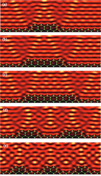
surface is a-type and flat and shows a maximum when the surface is b-type and flat. Fig. 10 shows CSEIs when the glancing angle is 2.56◦. Parts (a)
and (e) show CSEIs from b-type and a-type flat surfaces, respectively. The bright and dark lines in (a) are slightly curved and run nearly parallel to the surface. On the other hand, the CSEI from the a-type flat surface (e) shows a chequered pattern. The contrast along the central line normal to the surface and the contrast along the edge line are opposite to each other and bright and dark contrast appears alternately along the horizontal direction. The CSEI variations along the surface normal direction at the center, I(k,a/2,z), and those at the edge, I(k,0,z), are shown in the upper panel of Fig. 11. The intensity along the center and along the edge are almost in antiphase. The chequered pattern in (e) is similar to that shown in Fig. 5 (c), but in the present case the phase difference is caused by the atomic corrugation with one atomic layer normal to the incident beam azimuth.
Parts (b), (c), (d) and (f), (g), (h) of Fig. 10 show CSEIs for the non-flat stages of the growth cycle while Fig. 11 (center and lower panels) shows the corresponding intensities, Iav(k, z). The variations in the average amplitudes
of the oscillations are consistent with the specular beam intensity variations. The amplitude of the intensity variation decreases as the number of a-type atomic rows increases from 0 (a) to 12 (d) and shows a minimum for the a-type flat surface (e) when the step density is fixed (0.125). The amplitude then increases as the number of b-type atomic rows increases from 0 (e) to 12 (h). These variations explain why the systematic intensity variation in
the specular beam is observed.
The ratio of surface areas of the a-type and b-type surfaces changes as from 1/3 (b) to 1 (c) and then to 3 (d) in Fig. 10, and the specular beam intensity decreases as the contribution from the a-type surface increases. The decrease of the specular beam intensity can be explained by the contributions of waves with opposite phases showing a chequered pattern. It is found that Iav(k, z) obtained from Fig. 10 (c) and Isum(σn, z) calculated with n=8 show
excellent agreement as shown in Fig. 12 and this suggests that the disturbance caused by the step edges is small.
An intensity variation with a long period along the surface normal also occurs. This can be seen clearly in the upper panel of Fig. 11 where the rapid intensity oscillations show a modulation whose period is approximately 16 ˚A, about an order of magnitude greater than the basic oscillation period. The same modulation can be seen on close inspection of Figs. 10 (a) and (e). The phases of the longer period of the oscillation are opposite from one line to the next parallel to the surface both in (a) and (e). This longer period of oscilla-tion is caused by interference between the specularly reflected beam and the two adjacent diffracted beams in the zeroth Laue zone. The perpendicular component of the specular beam wave vector is about an order of magnitude bigger than the perpendicular components of the wave vectors of these two diffracted beams. This explains why the period of the modulation is about an order of magnitude larger than the basic period. The longer period of the modulation does not influence on the specular beam intensity appreciably when the number of atomic rows in the topmost layer changes. The change in the specular beam intensity is mostly caused by the relative contributions of the waves whose interference leads to the basic short oscillation period. 6. Discussion
The most important result of sections 4 and 5 is the relation between the form of the standing wave above the surface and the specular beam intensity. At the glancing angle of 1.22◦ the specular beam intensity is high when the
CSEI shows a standing wave with bright and dark contrast running almost parallel to the horizontal direction (a) and (e)-(h) in Fig. 5. The specular beam intensity shows a near maximum when the amplitude of the standing wave is nearly maximum as shown in curve (e) or (f) in Fig. 6. The change in the specular beam intensity is relatively small when a b-type island is formed on the a-type surface as shown in Fig. 2. The larger change occurs
(a) (e) (f) (g) (h) (b)
(c)
(d)
Figure 10: CSEIs from 16× 1 supercell surfaces with (a) 0, (b) 4, (c) 8 and (d) 12 a-type atomic rows on a b-type surface, and those with (e) 0, (f) 4, (g) 8 and (h) 12 b-type atomic rows on an a-type surface when the step density is fixed (0.125). The incident beam glancing angle is 2.56◦.
Av er ag ed E I ( ar b. u ni ts) Av er ag ed E I ( ar b. u ni ts) Distance (Å) 300 250 200 150 100 50 El ec tro n i nt en sit ies (a rb . u ni ts) 15 10 5 center edge 250 200 150 100 50 15 10 5 (e) (f) (g) (h) 250 200 150 100 50 15 10 5 (a) (b) (c) (d)
Figure 11: The upper panel shows CSEIs (I(k, x, z)) along the surface normal direction (z) at the center(x = l/2) and the edge (x = 0) of Fig. 10 (e). The center panel shows Iav(k, z) for CSEIs (a), (b), (c) and (d) in Fig. 10. The lower panel shows Iav(k, z) for CSEIs (e), (f), (g) and (h).
250 200 150 100 50 0 El ec tro n i nt en sit ies (arb. uits) 15 10 5 0 Distance (Å) (a) (b)
Figure 12: Comparison of average CSEI variations Iav(k, z) from a surface with a b-type island of 8 atomic rows formed on a flat b-type surface (a) with values calculated by using Isum(σn, z) in Eq. 7 with n=8 (b).
when an a-type island is formed on the b-type surface as shown from (b) to (d). The specular beam intensity shows a near minimum when a half of the a-type island is formed on the b-type surface (Fig. 5(c)). The association of high specular beam intensity with bright and dark contrast running parallel to the surface can be seen clearly in this data.
Similar correspondence between the specular beam intensity and the con-trast of the CSEI is found at other glancing angles. For example, at 2.56◦,
when the specular beam intensity shows a peak, the corresponding CSEI shows a standing wave with bright and dark contrast running almost parallel to the horizontal direction as shown in Fig. 10 (a). However, when the spec-ular beam intensity shows a near minimum, the corresponding CSEI shows a standing wave with bright and dark contrast appearing alternately in the horizontal direction which results in a chequered contrast (e).
The same correspondence occurs at all the glancing angles in Fig. 2. Fig. 13 illustrates this for the special case of flat surfaces. CSEIs are shown for flat a-type and b-type surfaces at glancing angles of 2.04◦, 2.56◦, 2.96◦ and
3.84◦. The data for 2.56◦ is the same as shown in Fig. 10 and is included for
comparison. It is clear that a contrast pattern of slightly curved stripes appears whenever the specular beam intensity is at a maximum or near maximum while chequered contrast appears whenever the specular beam intensity is at a minimum or near minimum. Thus when the surfaces are flat similar contrast patterns occur repetitively as the specular beam intensity goes through maxima and minima. In (e), the contrast near the surface is quite bright and shows a chequered pattern while it shows slightly curved
(a) (b) (c) (d) (e) (f) (g) (h)
nmax nmin nmin max max min min max
Figure 13: CSEIs from flat surfaces. (a) CSEI from the a-type and (b) the b-type flat surface at the glancing angle of 2.04◦. (c) and (d) are those from a-type and b-type surfaces at 2.56◦, respectively. (e) and (f) are those from a-type and b-type surfaces at 2.96◦. (g)
and (h) are those from a-type and b-type surfaces at 3.84◦. Maxima and minima in the
specular beam intensity are indicated with max and min respectively, near maxima and minima with nmax and nmin.
stripes in the upper region. This bright and chequered contrast is caused by a so-called surface resonance where grazing emergent beams 0±2 are excited in the crystal nearly parallel to the surface [16]. As the beams are localised near the surface the interference with the beams appears only in a limited region outside the surface.
The CSEIs at the glancing angles in Fig. 2 are also qualitatively similar when the surfaces are not flat. When the number of atomic rows in an island increases the variations in the specular beam intensity are the same at the glancing angles 2.56◦ and 3.84◦ (Fig. 2). The CSEIs from the a-type
and b-type flat surfaces at 2.56◦ are similar to the CSEIs at 3.84◦ as shown in Fig. 13, although the period of the variations along the surface normal becomes small as the glancing angle increases. At the glancing angles 2.04◦
and 2.96◦, the a-type surface plays the same role as the b-type surface at the glancing angles of 1.22◦, 2.56◦ and 3.84◦. But the correspondence between
the maximum of the specular beam intensity and the nearly parallel bright and dark contrast in the horizontal direction holds, and the correspondence between the minimum of the specular beam intensity and the chequered contrast also holds.
When epitaxial growth is monitored with RHEED, the incident beam glancing angle is usually chosen so the specular beam intensity shows a peri-odic oscillation as a function of growth time and has an intensity maximum or a near maximum from a starting flat surface. In this case we can expect that bright and dark contrast in the CSEI runs almost parallel to the sur-face at the initial stage. Then there are two possible origins of the RHEED intensity oscillation. One is the phase difference between two successive lay-ers such as the topmost layer and the adjacent underlying layer as shown in Fig. 5 and Fig. 10. The other is the disturbance of the CSEI caused by steps as shown in Fig. 8. The specular beam intensity variations from surfaces of an island of monolayer height belong to the former case. On the other hand, the specular beam intensity variations that occur when the number of atomic rows is fixed and the number of islands of biatomic height changes belong to the latter case.
In this paper, we have assumed that the substrate crystal has a single domain Si(001) surface and we have focussed on understanding the physics of the RHEED intensity variations during growth of a single domain. However, in actual homoepitaxial growth on Si(001) the surface consists of two kinds of domains with steps of monolayer height (or a multiple of this height). It is difficult to calculate the RHEED intensities in this situation because it may be necessary to take account of multiple scattering of waves by different domains. However we have tried to estimate the effect of the domains by summing the intensities from surfaces of the same number of atomic rows of a-type and b-type on the b-type and a-type surfaces, respectively. The right hand panel of Fig. 2 shows the resulting variation of the specular beam intensity. There is a maximum from a flat surface at all the glancing angles in the left panel except at 2.04◦. That is, the specular beam intensity is a maximum at the start of the growth, except at 2.04◦.
In summary, the origin of RHEED specular beam intensity oscillations can be explained by two possible types of interference of electron waves inside and outside the crystal surface. One origin partly agrees with the two level interference model at an off-Bragg condition [2], although the present result is obtained around a peak position and based on a multiple scattering theory. In this case the origin is closely related to the atomic row density of the topmost layer. The other origin is related to the disturbance of waves by steps on the surface and to the difference ∆Istep. This origin partly agrees
with the step density model [8], but the model can be applied only to limited cases. This is because the primary origin is the change in the interference
between waves from two different levels and the disturbance of the waves by steps becomes dominant only when the change in this interference is small. In the present case, for a surface with biatomic height steps the change in the interference between waves from two different levels with a bilayer height step is small and the disturbance by steps becomes dominant.
7. Acknowledgment
This work is supported by KAKENHI (C) from Ministry of Education, Culture, Sports, Science and Technology.
8. References
[1] J.H. Neave, B.A. Joyce, P.J. Dobson, and N. Norton: Appl. Phys. A31 (1983) 1.
[2] C.S. Lent and P.I. Cohen: Surf. Sci. 139 (1984) 121.
[3] T. Kawamura, P.A. Maksym, and T. Iijima: Surf. Sci. 148 (1984) L671. [4] T. Kawamura and P.A. Maksym: Surf. Sci. 161 (1985) 12.
[5] T. Kawamura: Surf. Sci. 351 (1996) 129.
[6] U. Korte and P.A. Maksym: Phys. Rev. Lett. 78 (1997) 2381. [7] J.D. Fuhr and P. M¨uller: Phys. Rev. B84 (2011) 195429. [8] S. Clarke and D.D. Vvedensky: Phys. Rev. B37 (1988) 6559. [9] T. Kawamura and P.A. Maksym: Surf. Sci. 601 (2007) 822.
[10] T. Kawamura and P.A. Maksym: Surf. Sci. Reports, 64 (2009) 122. [11] T. Kawamura and P.A. Maksym: J. Phys. Soc. Jpn. 78 (2009) 073601. [12] T. Kawamura and P.A. Maksym: J. Phys. Soc. Jpn. 80 (2011) 063602. [13] P.A. Makysm and J.L. Beeby: Surf. Sci. 110 (1981) 423.
[15] T. Sakamoto, T. Kawamura and G. Hashiguchi: Appl. Phys. Lett. 48 (1986) 1612.