平成23年（2011年）東北地方太平洋沖地震以降に活発化した福島県浜通りから茨城県北部における地震活動の特徴とその要因

平成

23 年（2011 年）東北地方太平洋沖地震以降に活発化した

福島県浜通りから茨城県北部における地震活動の特徴とその要因

Characteristics and Factors of the Earthquakes around the Northern Ibaraki Prefecture and the Coastal

Area of Fukushima Prefecture after the 2011 off the Pacific Coast of Tohoku Earthquake

武藤大介

，上野 寛

，溜渕功史

，岩切一宏

Daisuke MUTO

, Hiroshi UENO

, Koji TAMARIBUCHI

, and Kazuhiro IWAKIRI

(Received June 24, 2013: Accepted April 22, 2014)

ABSTRACT: Earthquakes have occurred actively around northern part of Ibaraki Prefecture and coastal area

of Fukushima Prefecture since the 2011 off the Pacific coast of Tohoku Earthquake (MW9.0). Most of these

earthquakes had the normal fault mechanisms, which was unusual for inland eastern Japan. At the largest event of the earthquake activity, two fault planes slipped: Shionohira Fault and Yunodake Fault. The time lag of these origin times between both fault slips was calculated to be about 5.9 seconds. We analyzed the source process of six major events, including the largest event, with near-field strong motion waveforms. Then, the SAR interferometly (InSAR) image and the hypocenters distribution of aftershocks were considered for setting fault plane parameters. The result of the largest shock was adjusted by some field survey reports. The moments of both fault planes of the largest events were roughly the same, though the surface displacement amount of Shionohira Fault was larger than that of Yunodake Fault, because the main slip area was located in the shallow zone on Shionohira Fault, whereas it was in the deeper zone on Yunodake Fault. Based on these fault models, ΔCFFs from the previous to the next event’s fault plane were solved, and each event occurrence was explained as viewed from ΔCFF. Additionally, we tried stress tensor inversions by the fault parameters for the source process analysis and CMT mechanisms, explaining the relationship between this activity and stress changes by the MW9.0 event. There are some examples of similar cases which are not limited to Japan:

inland seismic activities appear in particular areas after megathrust earthquakes, making it necessary to more carefully reveal the universality of the relationship between megathrust earthquakes and inland activities.

1 はじめに 2011 年 3 月 11 日に発生した平成 23 年（2011 年） 東北地方太平洋沖地震以降，福島県浜通りから茨城 県北部にかけての地域で，地殻内の地震活動が活発 化した．この地域で発生した最大の地震は 4 月 11 日17 時 16 分に発生した MJ7.0（MW6.7）の地震（以 下，本震と呼ぶ）で，福島県いわき市をはじめ2 県 4 市町村で最大震度 6 弱を観測する等した．この地 震を含め，2011 年中に最大震度 5 弱以上を観測する 地震が15 回発生する等，きわめて活発な活動が見ら れた． 本震により，福島県いわき市では明瞭な地表断層 を生じた．現地での調査結果によると，従来知られ ていた井戸沢断層の変位は小さく，その西側に平行 して走る断層（この地震以後，塩ノ平断層と呼称さ れることがある．たとえば石山・他，2011 等．本論 でもそのように呼ぶ）と，それに斜交する湯ノ岳断 層に沿って地表変位が認められた（阿南・他，2011； 堤・遠田，2012）．合成開口レーダー（SAR）による 干渉解析（安藤，2012；Kobayashi et al., 2012）でも， 2 つの明瞭な地表断層が見られる．そこで，これら を説明する断層モデルの提案を試みる． 今回の地震活動が発生した地域はこれまで目立っ た地震がほとんど知られておらず，東北地方太平洋 沖地震により地震活動が励起されたと考えられる． また，東日本の地殻内としては珍しく，正断層型の 地震が卓越していることも特徴として挙げられる． 遠田（2011）及び遠田（2012）はクーロン応力変化

1_{気象研究所地震火山研究部，Seismology and Volcanology Research Department, Meteorological Research Institute} 2_{地震火山部地震予知情報課，Earthquake Prediction Information Division, Seismology and Volcanology Department}

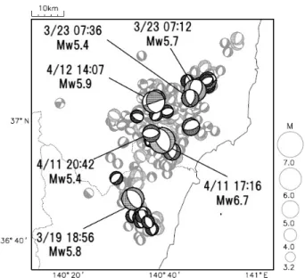
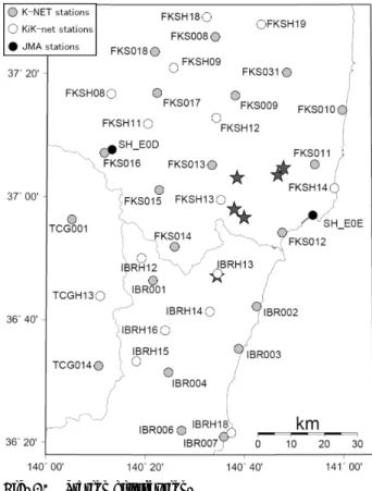
Fig. 1 Epicenter map and M-T diagram.

The earthquakes that were shallower than 20 km with MJ≥3.0 within 3 months from the origin time

of the 2011 off the Pacific coast of Tohoku Earthquake (14:46 on March 11 to June 11) were plotted on the map. The blue circles are the epicenters of events occurring before the main shock on April 11, while the red circles are those occurring after the main shock. The graph below shows the M-T diagram in the map area with colors identical to the map. Small dots with lengthwise lines indicate each event, and the sequential line graph shows the cumulative number of events.

（ΔCFF）から東北地方太平洋沖地震後の関東地方 の地震活動の説明を試みたが，本論では福島県から 茨城県の地震活動についても同様にΔCFF で説明が 可能かを検討する．また，応力テンソルインバージ ョンにより，今回の地震の活動領域の応力場を求め， 東北地方太平洋沖地震が周辺にもたらした応力場の 変化との関連についても議論する． 今回の地震活動は，東北地方太平洋沖地震の広義 の余震として取り扱われ，規模の割に注目度が小さ

Fig. 2 Comparison of aftershock activities of inland earthquakes in Japan.

The cumulative numbers of aftershocks are equal to or greater than MJ3.0. The chosen events are

various shallow inland earthquakes occurring since 1980 having JMA magnitudes of main shocks between 6.8 and 7.3. The horizontal axis denotes the time after the origin time of each main shock. Although the Mid Niigata Prefecture Earthquake in 2004 was generally known as an event with very active aftershocks, the number of aftershocks 60 days after this event was about 1.6 times that of the 2004 event. いと言える．しかし，死者5 人等の被害を生じる等， 防災上の観点からも無視できない．そこで，他のプ レート境界型巨大地震の発生後にも，今回の活動と 同じ特徴を持つ地震活動が発生した事例があるかに ついても調査した． 2 地震活動の概要 2.1 地震活動の特徴 2011 年 3 月 11 日 14 時 46 分に東北地方太平洋沖 地震が発生した直後から，福島県浜通りから茨城県 北部にかけての地域で地震活動が活発化した．3 月 19 日に茨城県北部で MJ6.1（MW5.8）の地震，3 月 23 日に福島県浜通りで MJ6.0（MW5.7）の地震，4 月11 日に福島県浜通りで MJ7.0（MW6.7）の本震，4

Fig. 3 Distribution of the focal mechanisms.

The focal mechanisms of earthquakes where the hypocenters were shallower than 20 km with MJ≥3.2 within 3 months from the origin time of the

2011 off the Pacific coast of Tohoku Earthquake (14:46 on March 11 to June 11) are plotted. The black ones are CMT, while the gray ones are the focal mechanisms estimated by P-wave initial motions. Most are normal types in every magnitude. 月12 日に福島県中通りで MJ6.4（MW5.9）の地震（以 下，最大余震と呼ぶ）が発生した．5 月以降も MJ5.0 以上の地震がしばしば発生した（Fig. 1）．MJ3.0 以 上の地震の回数は2011 年末までに約 1500 回に達し た．本震以降の60 日間に限っても 800 回近くに達し た．これは，とくに余震活動が活発であった平成16 年（2004 年）新潟県中越地震の余震回数を上回る（Fig. 2）． 活動領域は大きく 3 つに分けることが出来る．1 つ目は3 月 19 日 18 時 56 分の地震を中心とする茨城 県北部の領域で，東北地方太平洋沖地震の直後から 活動が活発化し，活動が長く続いている．2 つ目は 3 月23 日 07 時 12 分の地震以降に一時的に活発化した 領域である．3 つ目は本震を含む領域で，Fig. 1 を見 ても分かる通り，主に本震後に活発化した領域であ る． 2.2 発震機構解 今回の地震活動では，東北地方太平洋沖地震の発 生 直 後 を 除 い て ， 概 ね MW4.5 以上 の 地 震に つ いて

Fig. 4 Triangle diagrams of the focal mechanisms. Triangle diagrams of the focal mechanisms were prepared by CMT analysis with MW≥4.5 events

from March 11 to the end of 2011. We selected events (a) that occurred exclusively in the area of Fig. 1, (b) crustal events that occurred in eastern Japan (34 ° N < latitude < 41 ° N; 136 ° E < longitude <141 ° E; Depth < 20km) except aftershocks of the 2011 off the Pacific coast of Tohoku Earthquake and events occurring in the area of Fig. 1. CMT 解が，MJ3.2 以上の地震について初動発震機構 解が求められている．CMT 解と初動発震機構解の分 布をFig. 3 に示す． 今回の地震活動では，場所や規模を問わず正断層 型の地震が卓越している（Fig. 4(a)）．一方，MJ6 程 度以上の地震の中では，4 月 12 日の最大余震（MJ6.4， MW5.9）のみが正断層型とは異なる型であった．一 般に東日本の地殻内では逆断層型の地震や横ずれ断 層型の地震が卓越する（活断層研究会，1991）．今回 の地震活動を除く東日本の地震については，東北地 方太平洋沖地震後もこの傾向は変わらなかった（Fig. 4(b)）． 2.3 本震の震源断層と現地調査結果 本震の直後に行われた現地調査では，塩ノ平断層 と湯ノ岳断層の2 枚の断層に沿って変位が観察され た（たとえば，阿南・他，2011）（Fig. 5）．その変位 量は，塩ノ平断層で最大約2.1m（堤・遠田，2012）， 湯の岳断層で最大約0.8m（粟田・他，2011）に及ぶ． 両断層はほぼ同時に動いており（杉戸・他，2011）， 複雑な震源過程があったことが示唆される． 塩ノ平断層に平行な井戸沢断層の周囲でも，亀裂 や開口クラックが認められたが，その変位はせいぜ い 10cm 程度であり，塩ノ平断層や湯ノ岳断層に比 べて十分小さかったと言える（堤・遠田，2012）．そ のため，本論では井戸沢断層については考慮しない

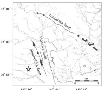
Fig. 5 Fault lines and outcrop distribution.

The circles drawn over the fault lines organized by Nakata and Imaizumi (2002) are outcrops reported by Wakisaka et al. (2011). The white star indicates the epicenter of main shock.

こととした． 3 本震の震源と断層パラメータ 3.1 得られたデータと特徴 塩ノ平断層と湯ノ岳断層の2 枚の断層面上で発生 した一連の地震の震源過程を解析する際には，両地 震の震源（各断層面上でのすべりの開始点）と断層 パラメータ（走向，傾斜角）を知る必要がある．今 回の地震では，気象庁一元化震源（検測値データを 含む），初動発震機構解及びCMT 解，SAR 干渉解析 により得られた面的地表変位等のデータが存在する ため，個々の長所を活用して，震源や断層パラメー タを決定する． 気象庁一元化震源は，計算に用いた速度構造等と 実際の速度構造等との差異に起因する系統誤差と， 相の読み取り誤差に起因するランダム誤差を含んで いる．しかし今回波形相関による相対走時を利用し た Double Difference 法（Waldhauser and Ellsworth, 2000；DD 法）を用いて震源再計算を行ったことで， 速度構造の差異に起因する系統誤差は軽減し，震源 の相対的な位置関係は精度が高くなる．そのため， 塩ノ平断層側と湯ノ岳断層側それぞれの震源の相対 位置や，余震分布の形状（Fig. 6）に使用することに した． 地表における断層位置は，現地調査結果が最も正

Fig. 6 The hypocenter distribution of aftershocks of the main shock relocated by the DD method.

The hypocenters of the earthquakes occurring from the origin time of main shock (17:16 on April 11) to 11:00 on April 13 were plotted. These were relocated by the Double Difference (DD) Method. The black circles indicate hypocenters of events occurring before the MJ6.4 event at 14:07 on April

12. The gray circles indicate hypocenters after the MJ6.4 event. The left figure below is a cross

section inside of pentagon on the map. The strike of the projection plane shown as A-B is set perpendicular to the strike of Shionohira Fault (N161°E). The seismic plane was noticed between two arrows. The right figure below is inside the rectangle, whose projection plane shown as C-D is perpendicular to the strike of Yunodake Fault (N128°E). Similarly the seismic plane was noticed between the arrows.

確であるが，空間的に連続してデータが得られてい

るわけではない．一方，SAR 干渉解析により得られ

た地表変位（安藤，2012）からは，地表断層全体の

位置及び走向を精度よく知ることができる（Fig. 7）． そ こ で 地 表 に お け る 断 層 位 置 と 走 向 に つ い て は ，

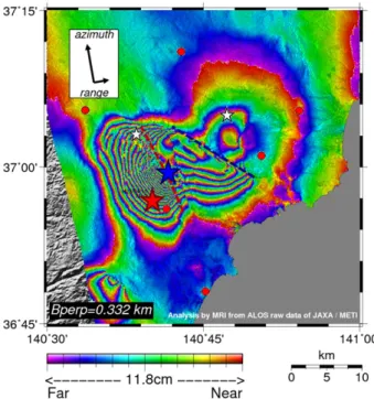
Fig. 7 The SAR interferometry image of hypocentral area of main shock.

The SAR interferometry image was analyzed using images photographed by ALOS (Ando, 2012). One image stripe shows an 11.8cm slide along the satellite’s line of sight. We can detect the fault line on the land surface of the main shock. The dark red line indicates Shionohira Fault, while the dark blue line indicates Yunodake Fault. The red star is the relocated epicenter, which is the rupture start point on the Shionohira Fault. The blue one is the rupture starting point on Yunodake Fault. The small white stars indicate the epicenters of the events occurring at 07:11 on March 23 and at 14:07 on April 12. Electric reference stations of the Geospatial Information Authority of Japan (GSI) are plotted as small red circles.

SAR 干渉画像の結果を採用した．なお，現地調査に より得られた地表断層の位置と，SAR 干渉画像によ り得られた地表断層の位置は，高い精度で一致する ことを確認した． 湯ノ岳断層側の断層すべりについては，その開始 点（震源）や時刻（発震時）は気象庁一元化処理で 求められていないが，独立行政法人防災科学技術研 究所のHi-net の波形（Fig. 8）からは湯ノ岳断層側の 断層すべりに伴う初動を見出すことが可能である． そこで， Hi-net と東北大学の計 14 点の波形（P 波 6 点，S 波 11 点）をもとに，新たに湯ノ岳断層側の震 源と発震時を求めた．さらに，塩ノ平断層側の震源 （気象庁一元化震源をもとに3.2 で示す手順 4 のと おり修正した震源）をマスターイベントにして，マ スターイベント法により，塩ノ平断層側の震源に対 する湯ノ岳断層側の震源の相対位置と時間差を求め た．Fig. 8 の(a)と(b)はそれぞれ，湯ノ岳断層側の震 源から南側と北側の波形を距離順に並べたものであ る．塩ノ平断層側の震源から発生した波と，湯ノ岳 断層側の震源から発生した波の時間差は，北側でよ り短い．つまり後者の震源は前者の震源よりも北方 に位置することが見て取れる．計算の結果，湯ノ岳 断層側の震源は塩ノ平断層側の震源の約 6km 北方 に，また両者の発震時の時間差は 5.9 秒と求められ た． 初動発震機構解及び CMT 解は，断層面の走向及 び傾斜角を決定する有力な手段である．しかし前者 は，断層すべりが開始された地点での断層パラメー タを表すもので，M6 を大きく超える地震における 断層面全体（この場合は塩ノ平断層全体）のパラメ ータを適切に表していない可能性がある．また後者 は，ひと続きに起きた地震全体の断層パラメータを 求めるもので，塩ノ平断層と湯ノ岳断層の2 つの断 層運動を含む今回の地震において，個々の断層のパ ラメータを知る手段としては適切でない．とくに本 震の CMT 解は，非ダブルカップル成分の大きさを 表すεの絶対値が0.39 と非常に大きい．つまり単純 な一つの断層面上の破壊でないことを示唆しており， やはり CMT 解から断層パラメータを引用すること は不適当と言える．そもそも今回の地震の断層面の 走向は，SAR 干渉画像や地表断層の調査によって正 確な値が得られるため，あえて発震機構解から走向 を決める必然性も小さい．そのため，今回の地震の 走向の設定に際しては，初動発震機構解及び CMT 解は参照しないことにした．断層面の傾斜角につい ては，後述のとおり余震分布から決定した値（57°） を採用したが，初動発震機構解の値（50°）につい ても解析を行い，観測波形をより説明できる前者の 値を最終的に採用した． GPS 基準局の変動については，地震の規模に対し てGEONET の観測網が粗く面的分解能が低いため， ここでは使用しなかった．また，現地調査で見つか った地表断層の傾斜角や線条痕（すべり角に相当） 等のデータもあるが，必ずしも断層面全体を代表す る値とは限らないため，これも採用しなかった． なお，Fig. 7 の SAR 干渉解析結果を見ると，赤い

Fig. 8 The waveforms of main shock.

UD component waveforms observed by Hi-net seismometers (NIED’s high-sensitivity seismograph network) are arranged in short-distance order from the hypocenter of the first shock corresponds to Shionohira Fault. The initial P and S waves excited by the first shock are highlighted in red with red arrows. In the same way, those due to the second shock corresponding to Yunodake Fault are highlighted in blue. Seven waveforms are shown in (a), which were observed at the stations north of the hypocenter; those at southern stations are shown in (b). These waveforms were reduced to 6.0 km/s by the hypocenter. The station map is (c). Station colors indicate the time lag between the initial times of P or S waves from the first shock and those of the second shock observed at each station.

Fig. 9 The fault model of main shock.

Two squares indicate the fault planes for source process analysis; intersection lines with the ground surface are represented by broken lines. Red and blue correspond to Shionohira and Yunodake segments. The stars on each fault indicate the hypocenters of both segments. Crosses near each segment’s intersection lines are outcrops reported by Wakisaka et al. (2011). Additionally, aftershock hypocenters occurring between main shock and largest aftershock relocated by the DD method are plotted.

(c)

(b)

(a)

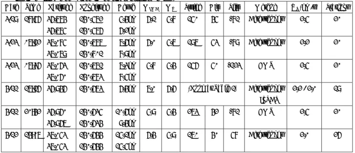
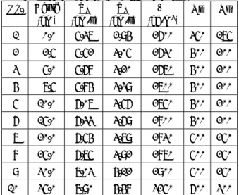
Table 1 Hypocenters and fault parameters of both segments of the main shock occurring at 17:16 on April 11.

These were relocated not only by the arrival time of seismic waveforms but also by the hypocenters distributions of aftershocks by the DD method and the ground deformation calculated by SAR interferogram analysis (Ando, 2012). Fault Time Latitude Longitude Depth Strike Dip Slip Fault length Fault width Shionohira 17:16:12.0 36.944° 140.667° 6.1km 161 57 -70 17.5km 15km

Yunodake 17:16:17.9 36.989° 140.696° 9.6km 128 51 -70 20km 15km

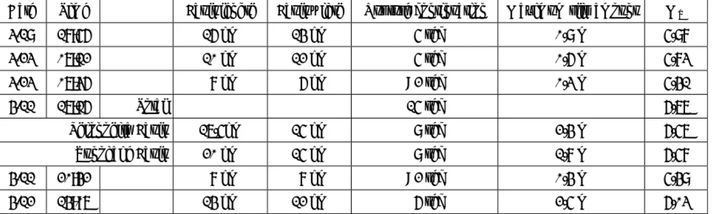
Table 2 List of events whose source processes were analyzed in this paper.

Dates and times indicate the origin time of each event. Latitude, longitude and depth in the upper half of each cell indicate the hypocenters of the JMA unified catalog; those in the lower half indicate the hypocenters relocated by the DD method. For the source process analysis described in this paper, hypocenters relocated by the DD method were adopted. MW was calculated by JMA centroid moment tensor analysis. Fault parameters (strike, dip, slip angle) for the

source process analysis were collected by the hypocenter distributions of aftershocks by the DD method or CMT analysis. Additionally, those methods were written. Furthermore the ground deformation calculated by SAR interferogram analysis (Ando, 2012) was used to estimate the fault parameters of the main shock. VR is the maximum

rupture velocity on the fault for the source process analysis. The numbers of stations in whose waveforms were used for inversion are described in the final cell of each row.

Date Time Latitude Longitude Depth MJMA MW Strike Dip Slip Method VR(km/s) Stations

3/19 18:56 36.784° 36.785° 140.572° 140.576° 5.4km 6.2km 6.1 5.8 150 45 -81 Aftershocks 2.5 20 3/23 07:12 37.085° 37.079° 140.787° 140.801° 7.6km 8.9km 6.0 5.7 197 53 -89 Aftershocks 2.2 20 3/23 07:36 37.063° 37.060° 140.771° 140.783° 7.3km 8.5km 5.8 5.4 156 50 -123 CMT 2.5 20

4/11 17:16 36.946° 140.673° 6.4km 7.0 6.6 (Look at Table 1) Aftershocks & InSAR 2.2 / 2.0 19 4/11 20:42 36.960° 36.967° 140.635° 140.634° 10.6km 9.4km 5.9 5.4 273 42 -81 CMT 2.5 20 4/12 14:07 37.053° 37.053° 140.644° 140.644° 15.1km 15.5km 6.4 5.9 170 40 58 Aftershocks 2.0 26 破線で示した塩ノ平断層の約2km 東にも，北北西－ 南南東に平行して走る地表断層があるように見える． これは井戸沢断層と考えられるが，本論では考慮し ていない． 3.2 震源と断層パラメータの推定 前節で触れた各データの特徴を踏まえ，震源と断 層パラメータを以下のとおり決定した： 1. SAR 干渉解析の結果（Fig. 7）から，塩ノ平断 層側の走向を決定する．また，断層面が地表面 と交わる位置も決定する． 2. 1 で決定した走向に直交するように断面を取 り（Fig. 6 の左下図），DD 法により得られた余 震分布から，断層面の傾斜角を決定する． 3. 1 で決定した地表での断層面の位置と，2 で決 定した傾斜角から，断層面の形状が決定される． 4. 波形相関 DD 法による再計算震源から断層面 に 下 ろし た 垂 線 が 断層 面 に 交 わ る点 を 震 源と 決定する． 5. 4.で求めた震源をマスターイベントとして， マスターイベント法により，湯ノ岳断層側の地 震の震源を再計算する． 6. SAR 干渉解析結果から，湯ノ岳断層側の走向 及び断層面が地表面と交わる位置を決定する． 7. 6 で決定した走向に直交するように断面を取 り（Fig. 6 の右下図），波形相関 DD 法により 得られた余震分布から，湯ノ岳断層側の断層面 の傾斜角を決定する．

8. 4 と同じく，6 で決定した地表での断層面の位 置と，7 で決定した傾斜角から，湯ノ岳断層側 の断層面が決定される． 得られた断層パラメータをTable 1 に，余震分布及び 地表断層との3 次元的な関係を Fig. 9 に示す．なお， 手順4 で計算される，塩ノ平断層側の断層面と再計 算震源との距離は 0.62km（水平方向に 0.52km，鉛 直方向に0.34km）であった．これは，再計算震源の 決定誤差（水平方向に0.49km，鉛直方向に 1.00km） にほぼ収まる．また，手順5 で求めた震源と，手順 6 で得られた地表での断層面の位置を満足するよう に，湯ノ岳断層側の断層面の傾斜角を求めることも できるが，その結果は51°であり，手順 7 で計算し た湯ノ岳断層側の断層面の傾斜角（51°）と矛盾し ない． なお，上述の手順では，断層面上におけるすべり 角を決定することはできない．現地調査（たとえば 阿南・他，2011）によれば，塩ノ平断層と湯ノ岳断 層はいずれも西傾斜の正断層であったことが分かっ ているため，ここではすべり角を-70°及び-90°で 計算して結果を比較し，両断層とも理論波形をより よく説明できる-70°を採用した． 4 本震及び主要な地震の震源過程 4.1 近地強震波形解析手法 本震及び概ねMJ5.8 以上の主要な地震について， 近地強震波形を用いた震源過程解析を行った（Table 2）．解析には，独立行政法人防災科学技術研究所の 強震観測網（K-NET），基盤強震観測網（KiK-net） 及び気象庁の震度観測点の加速度波形を用いた．観 測点は，各地震の震源との距離が近く（50km 程度 以下），かつ震源域からの方位角ができるだけ広がる ように選別を行った（Fig. 10）．各地震について，19 －26 観測点の 3 成分波形を取得し，波形データは， P 波到達から数十秒間の加速度波形記録を 1 回積 分し速度波形に変換した後，周期20 秒から 5 秒の バンドパスフィルターをかけて使用した．主要な余 震の断層パラメータは，波形相関を用いたDD 法に より再計算して得られた地震の震源分布から得た． 震源分布から明瞭な地震面が見えない場合には，気 象庁が求めた CMT 解を使用した．この場合，CMT 解の2 つの節面それぞれについて震源過程解析を行 い，観測波形をより良く説明できる側の節面を採用

Fig. 10 Station distribution.

The gray and white circles indicate the K-NET and KiK-net stations of NIED, respectively. The black circles indicate JMA stations. All stations for using source process analysis having at least one event have been plotted. Stars are the epicenters of the events listed in Table 2.

した．本震については 3.2 節の方法によった．断層 のすべり角の初期値は，地震の震源分布から断層面 パラメータを設定した場合も含め，気象庁 CMT 解 によった．また本震については，現地調査結果を参 考に-70°と-90°で計算し，観測波形をよく説明で きる-70°を採用した．なお解析では，すべり角の初 期値から±45°の範囲で自由度を持たせて解析する ため，数度程度異なる初期値を与えても結果にはほ とんど影響しない． また，断層面は，地震活動の震源の広がりを基に 矩形断層として設定した．解析の結果，設定した断 層面の中心付近でしかほとんどすべりが生じない場 合には断層面を小さく与え直し，逆に断層面の辺縁 部に大きなすべりが生じた場合は断層面を広く与え 直す等，断層面は適宜設定し直して解析した．地震 活動からは断層面の広がりが明らかでない場合も， まず適当な断層の広がりを与えたのち，適宜断層面

Table 3 Structure for the source process analysis. The upper boundary depths of each layer are shown. VP and VS are the velocities of P and S waves. ρ

and Q are the density and quality factors. VP, VS

and ρ are cited from Matsubara and Obara (2011). Suitable inland values were given to Q factors. In this analysis, Q factors have little effect on calculations because the lengths between the hypocenters and each station were short.

No. Depth (km) VP (km/s) VS (km/s) ρ (kg/m3₎ Qp Qs 1 0.0 5.37 2.94 2600 350 175 2 2.5 5.52 3.05 2630 400 200 3 5.0 5.68 3.20 2670 400 200 4 7.5 5.84 3.39 2700 400 200 5 10.0 6.07 3.56 2750 400 200 6 15.0 6.33 3.69 2800 400 200 7 20.0 6.54 3.79 2830 500 250 8 25.0 6.75 3.92 2870 500 250 9 30.0 7.03 4.12 2900 500 250 10 35.0 7.90 4.48 3250 600 300 を設定し直して解析を繰り返した．断層面全体を数 十の小断層に分割した．ただし，各小断層の大きさ は，走向方向，傾斜方向ともに2km 以上とした．全 ての小断層で走向，傾斜，すべり角の初期値は統一 されているが，すべり角は初期値から±45°の範囲 で小断層毎に異なる値を取りうるとした． 断層パラメータを設定の後，各小断層のすべり量 を求める際には，multiple time window 法を用いて， 時空間のすべり量が滑らかになるような制約を加え た イ ン バ ー ジ ョ ン を 行 っ た （ た と え ば ，Ide et al., 1996）．すべり量分布の滑らかさを規定するパラメー タの値はABIC が最小になるように選んだ（Fukahata et al., 2003）．すべり角は，CMT 解のすべり角から± 45 ° 以 内 に 収 ま る よ う に 拘 束 し た （ Lawson and Hanson, 1974）．各小断層のグリーン関数は，離散化 波数積分法（Bouchon, 1981）により，反射・透過係 数行列（Kennet and Kerry, 1979）を用いて計算した． 非弾性減衰の効果は武尾（1985）の方法により考慮 した．地震波速度構造はMatsubara and Obara（2011）

によって得られた構造を参考にし，Table 3 に示す水 平成層構造とした． 断層上ですべりが伝播する速度は，震源域がある 深さでのS 波速度の 7 割にあたる 2.5km/sec 以下と なるよう制約を課した．それでもなお，余震域に対 して解析で得られるすべり量の分布が広がりすぎる 場合や，モーメントの解放が震源近傍で長く留まる ことが示された場合は，同速度を2.0-2.2km/sec に設 定し直して解析した． 本震については，3.2 節で求めた断層パラメータ をもとに解析を行った．震源時に塩ノ平断層側に与 えた点ですべりが始まり，5.9 秒後に湯ノ岳断層側 に与えた点でもすべりが始まるとした．インバージ ョンについては，予め与えた断層パラメータを持つ 各小断層におけるモーメント解放の重ね合わせで表 現しているため，断層の形状が複雑になっても処理 は変わらない． 4.2 本震の断層モデルの推定と議論 本震の解析の結果をFig. 11-4 及び Table 4 に示す． 本震のうち，塩ノ平断層側の浅い場所で 2m 以上 のすべりが推定された．これは丸山・他（2012）や 堤・遠田（2012）が報告した地表断層の位置及び変 位量と概ね整合する．とくに，SAR 干渉解析結果（Fig. 7）では，南北に延びる塩ノ平断層の中央付近で地表 変位が大きいことが分かるが，本解析結果でも断層 面の中央上部付近で大きなすべりが得られている． 一方，湯ノ岳断層側のすべりは主に深い場所に求め られたが，これは湯ノ岳断層側では 1m を超える地 表変位は報告されていないことと符合する．両断層 上のすべりの規模はそれぞれMW6.57 と 6.58 であり， 同程度であった． 引間（2012）は本解析と同様に塩ノ平断層と湯ノ 岳断層を考慮して，近地強震波形から震源過程を解 析している．塩ノ平断層側は，震源のやや北の浅い 部分で 2m を超えるすべりを求めており，本論にお ける解析結果とよく一致する．しかし湯ノ岳断層側 のすべりの開始点は断層面北端に位置し，本論とは 異なる．また，引間（2012）の両断層上のすべりの 規模はそれぞれMW6.53 と 6.30 であり，塩ノ平断層 側は本論と同程度であるが，湯ノ岳断層側では本論 よりも小さくなっている． 引間（2012）は，周期 1.25～33 秒のバンドパスフ ィルターを使用しており，本解析（周期5～20 秒） よりも広い帯域の波形を使用しているが，両者の中 心周波数は概ね同程度であり，周波数の違いによる 顕著な結果の違いは想定しにくい．また，塩ノ平断

Table 4 Results of source process analysis.

Fault lengths and widths were obtained by inversion repeatedly; that is, fault planes were widely set at the start and were struck off sub-faults not contributing moment release gradually. Rupture continuations were defined as the period between the origin time (rupture start time) and the time the moment rate was about one-tenth of the peak. Each value of the main shock occurring at 17:36 on April 11 was described as two individual segments. Additionally, the rupture continuation and MW were described as chain fault movement of the main shock.

Date Time Fault length Fault width Rupture continuation Maximum slip amount MW

3/19 18:56 16 km 14 km 5 sec 0.9 m 5.98

3/23 07:12 10 km 12 km 5 sec 0.6 m 5.83

3/23 07:36 8 km 6 km <2 sec 0.3 m 5.41

4/11 17:16 Total 15 sec 6.77

Shionohira Fault 17.5km 15 km 9 sec 2.4 m 6.57

Yunodake Fault 20 km 15 km 9 sec 1.8 m 6.58

4/11 20:42 8 km 8 km <2 sec 0.4 m 5.49 4/12 14:07 14 km 12 km 6 sec 2.5 m 6.03 層側については，引間（2012）は傾斜角を本論より もやや高角の62°と設定しているが，その他の断層 パラメータは概ね本論と似通っている．そのため， 塩ノ平断層側のすべり量分布やモーメントは，本論 と引間（2012）がよく一致したものと考えられる． 一方，湯ノ岳断層側で両者の結果が異なった理由 としては，両断層面上でのすべり開始時刻の時間差 の違いが考えられる．時間差は，本論の 5.9 秒に対 して，引間（2012）は 8 秒に設定されている．全体 のす べ り継 続 時間 は 本論 ， 引間 （2012）とも約 15 秒とほぼ同じであるため，湯ノ岳断層側でのすべり 継続時間は本論では最大9 秒間継続しうるのに対し， 引間（2012）では 7 秒以下に制約された．その結果， 断層面の長さも本論の 20km に対して引間（2012） は14km と短くなっている．しかし，阿南・他（2011）， 脇坂・他（2011）によれば，湯ノ岳断層側の地表の 変位・変状が見られる範囲だけで 15.5km に及んで おり，震源過程を計算する際に，地表変位を生じな い断層端も含めた範囲として 14km を上限とするの は適当でないと考えられる．また，湯ノ岳断層上の すべりで解放されたモーメントは，本論では塩ノ平 断層側と同程度と求められたが，引間（2012）は塩 ノ平断層側の半分以下である．しかし近地強震波形 の短周期成分は，1 つ目の波群（おもに塩ノ平断層 側のすべりに起因）に対して，2 つ目の波群（おも に湯ノ岳断層側のすべりに起因）のほうが大きな振 幅が観測された地点があり，これも本論の解析結果 に有利である．引間（2012）は，この点に関して， 井戸沢断層側のほうが長周期成分の放出が多く，湯 ノ岳断層側では短周期成分の放出が多かったためだ と考察している． 4.3 その他の地震の断層モデル 本震以外の地震の解析結果を Fig. 11-1 から 11-6 （11-4 は本震）及び Table 4 に示す．6 地震全ての解 析において，観測波形と理論波形は概ね一致してお り，解析結果の精度は高いと考えられる． 3 月 19 日 18 時 56 分の地震（Fig. 11-1）は，その 余震が震源の南側に分布しているが，本解析で得ら れたすべり量分布も震源から南に広がっており整合 する．また，SAR 干渉画像（Fig. 7）によれば，断 層面の北側に対応する地域で干渉縞が多く地表変位 が大きいが，本解析結果でも断層面の北側ですべり 量が大きく整合的である． 3 月 23 日 07 時 12 分の地震（Fig. 11-2）は，その 余震が震源の南側に分布しているが，本解析結果で 得られたすべり量分布もそれと整合する．また，SAR 干渉画像によれば断層面の南側に対応する地域で地 表変位が大きいが，本解析結果でも震源から離れた 断層面の南側ですべりが大きいことが示された．ま た，同日07 時 36 分の地震によるすべり（Fig. 11-3） は，07 時 12 分の地震の震源とおもなすべり域のあ いだを埋める場所に位置することが示された． 4 月 12 日 14 時 07 分の最大余震（Fig. 11-6）は， 本震の余震域内に近接した場所で発生したため，断 層面の広がりと最大余震の二次余震の分布を厳密に

Time from origin time (sec)

(a)

_(c)

Fig. 11-1 Results of the source process analysis of the event occurring at 18:56 on March 19.

(a) The slip amount distribution on the fault. The contour interval is 0.1m. The sky blue colored crosses are the centers of sub-faults and the white star is the epicenter. The gray circles show the epicenters of events with MJ≥2.0 occurring

within 24 hours. (b) Moment rate functions. (c) Observed waveforms (black) and theoretical waveforms (red) at each stations. The three waveforms indicate the vertical, north-south and east-west components from the left. Vertical axes were set in individual stations according to peak amplitudes; scales (cm per sec) are shown on the right. Waveforms at 12 stations in near order from the epicenter are shown. (d) Mechanism. The adopted fault plane for analysis is highlighted in red and the parameters (strike, dip, slip) are described.

Fig. 11-2 Results of the source process analysis of the event occurring at 07:12 on March 23.

The forms of each figure are the same as Fig. 11-1. (a) The contour interval is 0.15m.

Time from origin time (sec)

(b)

(d)

(d)

(a)

(c)

(b)

Shionohira Fault Yunodake Fault

(c)

(a)

(c)

(b)

(e)

Fig. 11-3 Results of the source process analysis of the event occurring at 07:36 on March 23.

The forms of each figure are the same as Fig. 11-1. (a) The contour interval is 0.1m. The slip amount distribution of the event at 07:12 on March 23 is indicated by the dotted lines.

Fig. 11-4 Results of the source process analysis of the main shock occurring at 17:16 on April 11.

The forms of figure (a), (c) and (d) are the same as Fig. 11-1. (a) The contour interval is 0.4m. The light red star indicates the epicenter and the light blue star indicates the location where the rupture started on Yunodake Fault. (b) The moment release on Shionohira Fault is shown in red, while that of Yunodake Fault is shown in blue. The gray colored graph shows the total moment release. (e) Slip distributions on the faults seen from the front of each fault were put in because Yunodake Fault is hidden in (a). The arrows indicate the slip directions of the hanging walls as seen from footwalls. Time from origin time (sec)

(b)

(d)

(a)

(d)

(156, 50, -123)

(161, 57, -70) (128, 51, -70) Shionohira Fault Yunodake Fault

(a)

(b)

(c)

(a)

(c)

(b)

Fig. 11-5 Results of the source process analysis of the event occurring at 20:42 on April 11.

The forms of each figure are the same as Fig. 11-1. (a) The contour interval is 0.1m. The dotted lines indicate the slip distribution of the main shock.

Fig. 11-6 Results of the source process analysis of the largest aftershock occurring at 14:07 on April 12.

The forms of each figure are the same as Fig. 11-1. (a) The contour interval is 0.3m. The dotted lines indicate the slip distribution of the main shock.

Time from origin time (sec) Time from origin time (sec)

(d)

(273, 42, -81)

(d)

Fig. 12 ΔCFF on Yunodake Fault induced by the slip of Shionohira Fault

Coulomb Failure Function (ΔCFF) at 5.8 seconds after the origin time of slip on Shionohira Fault. Warm colors indicate ΔCFF plus, while cold colors indicate it minus. Brown squares represent the fault planes of Shionohira Fault and white circles are the points where the slips started on Yunodake Fault. (a) Result of calculation with frictional coefficient of 0.8. (b) That of 0.4. This value (per 10-6_{) was normalized with the modulus of rigidity in crust. If the}

modulus of rigidity was 30 GPa, ΔCFF needed to be multiplied by 3×1010_.

対応付けるのは困難である．しかし4 月 12 日 14 時 07 分以降 24 時間以内には，最大余震の南側で多く の地震が発生しており（Fig. 6），最大余震のすべり が南側に広がっていることと整合する． 5 今回の地震の発生要因 5.1 ΔCFF を用いた解釈 5.1.1 本震の湯ノ岳断層側のすべり 本震では，塩ノ平断層側のすべりによって生じた 応力変化が，湯ノ岳断層側のすべりを誘発した可能 性がある．ここでは静的応力変化（クーロン応力変 化：ΔCFF）によって，湯ノ岳断層側のすべりが説 明できるか検討を行った． 震源過程解析により得られた，湯ノ岳断層側のす べりが始まる直前（発震時から 5.8 秒後）までの塩 ノ平断層側のすべりモデルを用いて，湯ノ岳断層側 の断層モデルに与えるΔCFF を計算した．ΔCFF の 計算には Okada（1992）及び内藤・吉川（1999）に よる理論地殻変動解析ソフト（MICAP-G）を使用し た．媒質は半無限媒質を仮定し，法線応力に係る内 部摩擦係数は 0.4 及び 0.8 とした．また結果は剛性 率で規格化した値として表示した． 結果をFig. 12 に示す．ここでは剛性率で規格化し た値を10-6_{単位で示しているため，たとえば剛性率} を30GPa と仮定する場合は，図の値に 3×1010_を掛 ける必要がある． 内部摩擦係数を 0.4 として計算すると，湯ノ岳断 層側のすべりが始まった点はΔCFF が負の値となる が，これを0.8 と仮定するとΔCFF は正の値をとる． しかしいずれにせよ，湯ノ岳断層側のすべり開始点 はΔCFF の分布の正負の境界付近に位置することに は変わりない．本震の震源過程解析時に設定した小 断層の間隔は2.5km あるほか，震源位置にも数百メ ートル程度の誤差を含むため，震源過程解析の空間 分解能や震源決定精度を考慮すると，数百メートル 以上の空間的精度で厳密にΔCFF の正負を判定する ことは困難である． 引間（2012）も同様の検討を行っているが，本論 と同様に，内部摩擦係数を 0.4 にした場合には湯ノ 岳断層側のすべり開始点でΔCFF が負となり，同 0.8 のときはΔCFF が正になることが示されている．こ のことから，ΔCFF の検討から，本解析結果と引間 （2012）の断層モデルの優劣を判断することは難し い． なお，湯ノ岳断層でのすべりが誘発された理由と しては，ここで検討した静的応力変化だけでなく， S 波等による動的応力変化等も考えられるが，ここ では立ち入らない．

Fig. 13 Calculation of ΔCFF

These figures show the Coulomb Failure Function (ΔCFF) when each event occurred. For instance, the top left and center figures show ΔCFF which the 2011 off the Pacific coast of Tohoku Earthquake (MW9.0) and its afterslip since March 18

have affected the fault plane same as the fault parameters of the March 19 event (MW5.8). Similarly, the top right

figure shows ΔCFF for 07:12 on March 23 event (MW5.7) due to the preceding events. Warm colors indicate ΔCFF

plus, while cold colors indicate it minus. White circles represent the epicenters of each event and brown rectangles represent the fault planes. As in Fig. 12, this value (per 10-6_{) was normalized with the modulus of rigidity in crust.}

Table 5 ΔCFF on each event due to preceding events. The modulus of rigidity is assumed 30GPa in this table.

Date and Time ΔCFF Note 3/19 18:56 +5.0×105 _Pa

3/23 07:12 +6.8×105 _Pa

3/23 07:36 +6.7×105 _Pa

4/11 17:16 +5.6×105 _{Pa Main shock}

4/11 20:42 The hypocenter was located in the border zone between the plus and minus area of ΔCFF. 4/12 14:07 The hypocenter was located on

the border zone between the plus and minus area of ΔCFF.

5.1.2 一連の地震活動 東北地方太平洋沖地震が今回の地震に及ぼす影響 についても，ΔCFF をもとに検討を行った．水藤・ 他（2012）及び水藤・他（2011）により東北地方太 平洋沖地震の地震時すべりと余効すべりのモデルが 得られているため，これらが3 月 19 日 18 時 56 分の 地震に与えるΔCFF を評価した．次に，東北地方太 平洋沖地震（余効すべりを含む）と3 月 19 日 18 時 56 分の両地震が，3 月 23 日 07 時 12 分の地震に与え るΔCFF を評価した．以下同様に，それまでに発生 した地震が次に発生する地震に与えるΔCFF を順次 求めた． 3 月 19 日 18 時 56 分の茨城県北部の地震に対する ΔCFF を計算する際は，東北地方太平洋沖地震の地 震時すべりに加えて，3 月 18 日 03 時までの余効す べりモデルを使用した．以下，3 月 23 日 07 時 12 分 及び07 時 36 分の地震について計算する際は，3 月 22 日 03 時までの余効すべりモデルを，4 月 11 日以 降の地震について計算する際は，4 月 14 日 03 時ま での余効すべりモデルを用いた．なお，4 月 11 日か ら見て 14 日は未来の時刻にあたるため，4 月 14 日 までの余効すべりモデルから4 月 11 日の地震に対す るΔCFF を求めるのは厳密には適切でないが，4 月 11 日から 14 日の間に余効すべりモデルに大きく影 響するような地震等は発生しておらず，以後の議論 には影響を与えないと考えられる． ΔCFF の計算は 5.1.1 と同様に行った．内部摩擦 係数は0.4 とした．解析結果を Fig. 13 及び Table 5 に示す． 東北地方太平洋沖地震は，東北地方の地殻内にあ

Fig. 14 The focal mechanisms used for stress tensor inversion.

The mechanisms colored red and blue were used for stress tensor inversion. The earthquakes for which fault models were obtained in this report are painted red and the other earthquakes are painted blue. The gray earthquake (maximum aftershock) was excluded from the inversion.

Fig. 15 Stress status and principle stress axes.

Stress states of MW≥4.8 events drawn by the red

and blue mechanisms in Fig. 14. Stereograms drawn as large circles are the lower hemispheres. The small squares in each stereogram show each stress state. The positions of small squares indicate σ₁ or σ3 orientation. The colors of each square

indicate stress ratio in 0.1 intervals. The tails on the left stereograms indicate the azimuth and the plunge angles of the stress statue of σ3 from that

of σ1. Those on the right stereograms indicate

those of σ1 from those of σ3. The red circles

show the representative directions that the variances of misfit angles were minimal.

る概ね南北方向に節面を持つ正断層型の断層面に対

して大きな正値のΔCFF を与えた（平塚・佐藤，2011）．

0.5-0.7MPa の正値をとる．地球潮汐による地殻応力 の 日 変 化 は お よ そ 103_{Pa オーダーと言 われており} （たとえば鶴岡，1995），ΔCFF はその数十倍に及 ぶことから，いずれもクーロン応力の変化で説明可 能である．本震以降の地震については，本震による 応力変化も大きく影響する．4 月 11 日 20 時 42 分の 地震及び4 月 12 日の最大余震の震源は，いずれもそ れらの地震の持つ断層パラメータに対するΔCFF の 分布における正負の境界付近にあった．5.1.1 でも述 べたとおり，数百メートル以上の空間的精度でこれ らのΔCFF の正負を判定することは，困難である． しかし，いずれについてもΔCFF からも説明できる 可能性を残している． 5.2 起震応力場 5.2.1 応力テンソルインバージョン 福島県から茨城県での地震活動の起震応力場を調 査するために，気象庁 CMT 解を用いた応力テンソ ル イ ン バ ー ジ ョ ン を 実 施 し た ． 解 析 に は ，Yamaji （2000），Otsubo and Yamaji（2006）による多重逆解 析法を用いた． 福島県から茨城県にかけて，概ねFig. 1 の範囲内 で東北地方太平洋沖地震の発生から3 ヶ月間に発生 した地震の CMT 解を用いて解析を行った．なお， 以降の解析では地震の規模による重みづけを行わな いため，より規模の小さな地震まで含めると，相対 的に小さな地震の応力状態に結果が左右される可能 性が増し，本活動領域全体の応力場の推定として適 切な値が得られなくなるおそれが生じる．現に規模 の下限を設けずに以降の解析を行った結果，満足な 結果が得られなかった．そこで，本震の規模（MW6.7） とのマグニチュードの差が 2.0 未満の地震（MW4.8 以上）に限って解析に用いることにした．なお，5.1.2 で述べたとおり，東北地方太平洋沖地震及びその余 効変動が最大余震に与えるΔCFF は負となり，最大 余震は本震による局所的なクーロン応力変化がなけ れば発生する可能性が低かったと考えられる地震で ある．つまり，東北地方太平洋沖地震による広域的 な応力場の変化と今回の地震活動の関係を議論する 際に，最大余震を解析対象に加えることは不適当で あることから，対象から外した．解析に用いた地震 は11 地震である（Fig. 14）が，本震は塩ノ平断層側 と湯ノ岳断層側双方を解析対象としたため，実質的 には12 地震である．震源過程解析を行った 6 地震（本 震は2 つの断層面それぞれを 1 つの地震と数える） についてはTable 2 に示した断層パラメータを用い， それ以外の6 地震については CMT 解を用いた． まず，実質12 地震の発震機構解をもとに，各地震 の応力状態を表示した（Fig. 15）．なお，Table 2 の 断層パラメータを用いた地震については，本来は共 役な断層面について考慮する必要はないが，解析の 都合上，Table 2 で示した値に加えて，それと共役な 断層面の値を求めて使用した．図で左側が最大応力 圧縮軸（σ₁）に，右側が最小応力圧縮軸（σ₃）に 対応する．ここで応力状態とは，任意に選びだした 5 つの断層面の組（全 12 地震の発震機構解の持つ 24 断層面の部分集合をなす．ただし同じ地震の両断層 面を選ぶことはできない）をもっともよく説明でき る応力場（応力軸とその応力比）のことである．こ こで，選んだ5 つ全ての断層面の断層パラメータを 満足する応力場が決められることが前提である．具 体的には，5 つそれぞれの断層面に対して，応力場 から期待される剪断方向（すべり角）と実際のすべ り角 の 差 が 20°の範囲で決められない組は除外さ れる．また，断層面の数を5 つとしているが，これ は応力テンソルインバージョンの解が安定するとし てYamaji et al.（2011）が推奨した数である．ただし， 断層面の組は 5 12 5 2 C すなわち25,344 通りあるため， 除外された組を考慮しても，得られる応力状態のパ ターンは多数に及ぶ．そこで，得られた個々の応力 状態を，60,000 パターンの応力状態のどれかに当て はめていき，15 以上の応力状態が重複したパターン だけをFig. 15 に表示している．結果として，より多 くの地震を説明できる応力状態だけが図に表示され ることになる．プロットされている小さな四角形は 検出された応力状態を示している．色の違いは応力 比Φ



 



















ここではさらに，12 個の地震の持つ断層パラメー タを全て説明できるσ₁軸及びσ₃軸を求め，応力場 を明らかにした．解の評価は，CMT 解（震源過程解 析を行った地震については得られたその結果）で得 られているすべり角と，解析で得られる応力場から 期待される剪断応力の方向との差（ミスフィット角） により評価した．CMT 解では 2 節面のうちどちらが 断層面に対応するか分からないので，どちらか片方 の節面でミスフィット角が20°以下であれば，その 地震の発震機構解は，得られた応力場から説明でき るものとみなした．震源過程解析を行った6 地震に ついては，震源過程解析で仮定した面についてのミ スフ ィ ッ ト角 が 20°以下であるように制約を課し た．全10 地震のうち出来るだけ多くの地震について ミスフィット角が20°未満となり，かつ各地震のミ スフィット角の自乗平均が最も小さくなる応力場を 最適解とみなした． 解析の結果得られたσ₁軸及びσ₃軸を，Fig. 15 に 大きな赤い円で示す．その値と応力比を以下に示す． σ₁：(azimuth, plunge) = (317°, 84°) σ₃：(azimuth, plunge) = (213°, 1°) σ₂：(azimuth, plunge) = (123°, 6°) Φ：0.4 求めた主応力軸を見ると，3 月 23 日 07 時 36 分に 発生した MW5.4 の地震のミスフィット角は 23°で あったが，それ以外の地震のミスフィット角は20° 以下であった．3 月 23 日 07 時 12 分の地震（ミスフ ィット角18°）と 07 時 36 分の地震（同 23°）及び 4 月 11 日 20 時 42 分の地震（同 20°）は，σ3軸が 東 北 東-西南西方向にあるときにミスフィット角が 小さくなる．両地震の震源を含む活動領域の北東部 では，それ以外の地域とはσ₃軸がやや異なってい た可能性がある．しかしいずれにせよ，大局的には σ₃軸は少なくとも南北方向ではないことが分かっ た． 5.2.2 周辺の構造線とのテクトニックな関係 今回の地震活動の発生要因については様々な解釈 が な さ れ て い る ． た と え ば ， 産 業 技 術 総 合 研 究 所 （2011）は，東北地方太平洋沖地震の余震分布から， 福島県から茨城県にかけての地域に分岐断層がある と推定し，この分岐断層がすべった場合に，周辺で 引っ張りの差応力が生じるとした．川邉・中野（2011，

Fig. 16 Earthquake activities since 1885.

A map of the earthquakes whose depths are shallower than 30 km. The gray symbols indicate epicenters of earthquakes occurring before the 2011 off the Pacific coast of Tohoku Earthquake, while the black symbols indicate those occurring after. 2012a，2012b）は，東北地方太平洋沖地震によって 東北地方が東西に伸長したことで，既存の断層や節 理の割れ目が広がったことに着目している．特に福 島県から茨城県にかけての地域は，内陸の浅発地震 面が海寄りにやや傾斜していることに着目し，東北 地方の伸長に伴って同地域が太平洋側へ重力的に滑 動した可能性を指摘した． とくに川邉・中野（2012a）では，本活動領域周辺 で割れ目が開口し，それに伴う地下水位の低下を指 摘している．このことは，5.2.1 で求めた応力場とし て，σ₁ 軸が上下方向にあることと調和的である． また川邉・中野（2011）は，地殻内の割れ目は既存 の地質構造に依存して生じるものであるから，東北 地方太平洋沖地震によって生じた東北地方南部から 関東地方にかけての広域的な伸長ひずみの方位と， 生じた割れ目は，必ずしも直交する必要がないこと を示している．このことは，5.2.1 で得られたσ3軸 が地域により多少ばらつきがあることを説明しうる． ただしその割れ目は同地域が東方向に滑動したこと に よ る 東 西 伸 長 を 原 因 と す る た め ， σ₃軸 が 南 北 方

Fig. 17 Schematic depiction of strain changes in the Tohoku region before and after the MW9.0 event.

(a) Steady strain changes before the 2011 off the Pacific coast of Tohoku Earthquake (the MW9.0 event). Because of

the subduction of the Pacific Plate and the coupling between the Pacific Plate and the land plate, the land had been compressed. Therefore, compressive strain had been accumulated in the northern and mid Tohoku region. In south-eastern Tohoku region including Fukushima Prefecture, little strain change had been observed. (b) Strain changes by the MW9.0 event. Compression of land plate was released and the strain changes of the land converted E-W

extension. These figures are referred to GSI (2008, 2011). However lengths and directions of arrows of these figures are qualitative, not strict.

向では説明がつかない．5.2.1 で得られたσ3軸は少 な く と も 南 北 方 向 で は な い こ と が 示 さ れ て お り ， 5.2.1 で得られた応力場は川邉・中野（2011）の説明 と矛盾しない． 5.3 東北地 方南部から 関 東地方にか け ての地域 で 活動が活発化した理由 国土地理院（2011）は GPS 連続観測記録をもとに， 2010 年 4 月と 2011 年 4 月のデータから，日本列島 のひずみ変化を求めている．東北地方太平洋沖地震 により，東北地方南部から関東地方北部にかけての 地域（概ね北緯 36-38°）では，概ね東西方向に顕 著 な 伸 長 ひ ず み が 生 じ た ． 東 北 地 方 の 概 ね 北 緯 38-40°の範囲では，ひずみ変化の伸長軸が北西－南 東方向にある．一方，平成 20 年（2008 年）岩手・ 宮城内陸地震発生前の，2007 年 4 月から 2008 年 4 月にかけてのひずみ変化（国土地理院，2008）が東 北地方の定常的なひずみ変化を示していると仮定す ると，北緯36-38°の地域ではひずみ変化は小さく， 同 38-40°の範囲では東西圧縮のひずみ変化があっ たと考えられる． もし東日本の地殻内のひずみは定常的なひずみ変 化の蓄積で表わされると仮定すると，北緯 38-40° の範囲では東西方向に圧縮軸を持つひずみが蓄積し ていたことになり，2003 年 7 月 26 日の宮城県中部 の地震や，平成 20 年（2008 年）岩手・宮城内陸地 震等は，ひずみを解放する運動として説明できる． 一方で，東北地方南部から関東地方北部にかけての 地域では，東北地方北部に比べてひずみの蓄積が小 さいために顕著な起震応力場が形成されず，東北地 方太平洋沖地震以前の過去100 年以上にわたり，地 殻内で MJ6.5 以上の顕著な地震は発生していなかっ た（Fig. 16, 17(a)）． 東北地方太平洋沖地震の発生により，北緯38-40° の範囲では，北西－南東方向に張力軸を持つ大きな ひずみ変化が生じ，同地域で蓄積されていたひずみ の一部が解放されたと考えられる．そのため，同地 域の地殻内では，以前より東西方向に圧力軸を持つ 逆断層型の地震が発生しにくくなっていると予想さ れる．現に同地域において，東北地方太平洋沖地震 の発生から2011 年末までに発生した MJ4.0 以上の地 震は以下のものに限られる（Fig. 18）： (i) 東北地方太平洋沖地震の発生から 6 時間以内 に発生したもの（1 個）：東北地方太平洋沖地 震 の 地 球 自 由 振 動 に 励 起 さ れ た 可 能 性 等 が 考えられるため，必ずしもひずみ変化や応力

Fig. 18 Epicenter map of shallow earthquakes and focal mechanisms around the Tohoku region.

The MJ≥4.0 earthquakes from 1995 to the end of

2011 were plotted on the map that the depths of the hypocenters were shallower than 20 km. The gray circles indicate the epicenters of events occurring before the 2011 off the Pacific coast of Tohoku Earthquake (the MW9.0 event) and the black circles

indicate those occurring within 6 hours of the MW9.0 event. The gray circles indicate those

occurring 6 hours or more after the MW9.0 event.

The focal mechanisms are the results of CMT calculations. If CMTs could not be analyzed, focal mechanisms calculated by particle motions were plotted. The dotted-line’s rectangle is the area of Fig. 1. 状態から説明できなくとも構わない (ii) 平成 20 年（2008 年）岩手・宮城内陸地震の 余震（1 個）：余震域のローカルなひずみ変化 も反映していると考えられるため，必ずしも 東北地方全体のひずみ変化や応力状態から説 明できなくとも構わない (iii) 秋田県（Fig. 18 の橙色の枠内）で発生した地 震（5 個）：発震機構解が求められた地震の解 は い ず れ も 北 西 － 南 東 方 向 に 張 力 軸 を 持 つ 型であり，東北地方太平洋沖地震後のひずみ 変化を反映している可能性がある 一方，北緯 36-38°の範囲では，東西圧縮のセン スを持つ定常的なひずみの蓄積が小さかった．その ため，東北地方北部に比べれば，もともと張力軸を 持つ地震が発生しやすい環境にあった．東北地方太 平洋沖地震により東西方向に張力軸を持つ大きなひ ずみ変化が生じたことにより，東西方向に張力軸を 持つ地震がより発生しやすくなった可能性がある． 今回の地震活動はこの応力変化により説明できる可 能性がある（Fig. 17(b)）． 6 今回の地震活動の普遍性に関する検討 6.1 陸羽地震との比較 今回の地震活動と同様に，プレート境界型の巨大 地震発生後に内陸の地殻内で顕著な地震が発生する 例がある．このうち，今回の地震と同様に，日本付 近のプレート境界で MW8 程度以上の地震が発生し たのち数ヶ月以内に，その震源域から概ね300km 以 内の内陸の地殻内でMW6.5 程度以上の地震が発生し た地震と比較を行った．該当する地震として，1896 年の明治三陸地震の約2 ヶ月半後に発生した陸羽地 震と，1944 年の東南海地震の約 1 ヶ月後に発生した 三河地震がよく知られている（たとえば，吾妻，2011）． 陸羽地震は1896 年 8 月 31 日 17 時 06 分に発生し た M7.2 の地震であり，秋田や神宮寺では烈震とな った（中央気象台，1897）．山崎（1896，1897）らの 調査によると，明瞭な地表断層（逆断層）を生じた． 本震に先立ち8 月 23 日頃から活発な前震活動が見ら れ，8 月 23 日 15 時 56 分と 8 月 31 日 16 時 42 分に 強震を記録している．秋田では，8 月 31 日に 53 回， 9 月 1 日に 49 回の揺れを記録する等の余震活動があ った． 陸羽地震は，顕著な前震活動を伴った点で今回の 地震に似ているが，前震が始まったのは明治三陸地 震から2 ヶ月以上経過した後であり，仮に誘発地震 だとすれば，2 ヶ月間地震活動がなかったことが説 明しづらい．

また，Tanioka and Satake（1996）による明治三陸 地震の断層モデルから，陸羽地震の断層面解に及ぼ す ΔC F F を 求 め た ． 陸 羽 地 震 の 断 層 面 解 は 山 崎 （1896）の報告や，松田・他（1980）等の研究も踏 まえて，走向210°，傾斜角 60°，すべり角 90°に 設定した．陸羽地震の震源の深さは5km と仮定した が，これより多少浅くあるいは深くしても，陸羽地 震の震源域周辺における結果は大きく変わらないこ とを確認した．媒質は半無限媒質を仮定し，摩擦係

Fig. 19 ΔCFF on the Rikuu Earthquake due to the Meiji Sanriku Earthquake.

This value (per 10-6_{) is normalized with the}

modulus of rigidity. If the modulus of rigidity was 30 GPa in the crust, ΔCFF must be multiplied by 3×1010_{. For instance, around the epicentral area of}

the Rikuu Earthquake, which is enclosed in a red circle, the value in this figure is about -3×10-7 _and

ΔCFF is about -9×103_{Pa. The fault model of the}

Meiji Sanriku Earthquake by Tanioka and Satake (1996) was adopted. The fault parameters for the Rikuu Earthquake were set to 210deg. of strike, 60deg. of dip, and 90deg. of rake with reference to Yamazaki (1896) and Matsuda et al. (1980). 数は0.4 とした．結果を Fig. 19 に示す．5.1 におけ る計算と同様に，図中の値は剛性率で規格化したも のである．仮に地殻内の剛性率が30GPa とすればΔ CFF は負（-9×103_{Pa 程度）となり，広域の応力変化} では陸羽地震の発生は説明がつかないことが示され た．明治三陸地震と陸羽地震の関係については，今 回の福島県浜通りから茨城県北部における地震活動 のような特徴は見られなかったと言える． 6.2 三河地震との比較 三河地震は1945 年 1 月 13 日 03 時 38 分に発生し たMJ6.8 の地震であり，震源周辺で住家の全壊率が 60%を超える等，強い揺れを生じた．深溝断層と横 須賀断層の2 つの断層に沿って明瞭な地表断層を生 じた．震源域周辺では，前年の 12 月 8 日に MJ4.5 の地震が発生する等，地震活動が活発化し，1 月 11 日14 時 57 分には MJ5.7 の前震が発生した．余震活 動も極めて活発で，30 日間に MJ4.5 以上の余震が 45 回観測された．これは2011 年 4 月 11 日に発生した

Fig. 20 ΔCFF on the Mikawa Earthquake due to the Tonankai Earthquake.

The normalization method is the same as that for Fig. 19. The red circle indicates the epicenter of the Mikawa Earthquake. The fault model of the Tonankai Earthquake by Yamanaka (2006) and the fault parameters for the Mikawa Earthquake by Takano and Kimata (2009) were adopted. ΔCFF around the hypocenter of Mikawa earthquake was about +0.06MPa when the modulus of rigidity was 30GPa in the crust.

今回の地震（30 日間に MJ4.5 以上の余震を 47 回観 測）に匹敵する．三河地震は，1944 年 12 月 7 日の 東南海地震の発生直後から周辺で地震活動が活発化 しており，余震活動が極めて活発であった点で，今 回の地震と共通する． 6.1 と同様に，東南海地震が三河地震の断層モデ ルに及ぼすΔCFF を求めた．東南海地震については，

Kanamori （1972），Ando（1975），Inouchi and Sato （1975），相田（1979），藤井（1980），Ishibashi（1981）， Iwasaki（1981），Sagiya and Thatcher（1999），Kikuchi et al.（2003），Ichinose et al.（2003），谷岡・馬場（2004），

山中（2004, 2006）等の断層モデルが知られている

が，ここでは近地強震波形をもとに Kikuchi et al.

（2003）の問題点を解決した山中（2006）のモデル

を採用した．三河地震については，Ando（1974）， 浜田（1987），Kakehi and Iwata （1992），山中（2004），

青木・他（2005），高野・木股（2009）等の断層モデ

ルがあり，ここでは余震分布と地表変位の両方を最

もよく説明する高野・木股（2009）のモデルを採用

Fig. 21 Aftershock activities of the Maui Earthquake in Chile (MW8.8).

The M≥4.5 earthquakes in which the depths of hypocenters were shallower than 100 km within 60 days from the origin time of the Maui Earthquake in Chile (15:34, February 27 to April 27 on JST) were plotted on the map. The blue circles indicate the epicenters of events occurring in the small rectangular area. The graph below shows the time series of events occurring in the large dotted rectangular area on the map. The colors have the same meanings as those on the map. Small dots with lengthwise lines indicate each event. The solid black line is the cumulative number of events occurring in small rectangular area on the map painted blue. The dotted brown line shows it occurred in large dotted rectangular area except in the small rectangular area painted red. Additionally the focal mechanisms of MW>6.5 earthquakes are

shown. Although the focal mechanisms of the main shock (MW8.8 event), the March 5 event, and the

March 16 event were thrust type, those of two events occurring in small rectangular area were normal fault type. Hypocenters and focal mechanisms were obtained by USGS PDE (Preliminary Determination of Epicenters) and Global CMT.

Fig. 22 ΔCFF on two inland earthquakes due to the Maui Earthquake in Chile (MW8.8).

The normalization method is the same as Fig. 19. (a) is the figure about the MW6.9 earthquake

occurring at 23:39 on March 11 and (b) is about the MW7.0 one occurring at 23:55 on the same day. The

white circles in each figure indicate the epicenters of the inland earthquakes. The fault model of the Maui Earthquake by JMA (2010) and the fault parameters of inland earthquakes by Global CMT were adopted. The fault planes for analysis are highlighted in red. ΔCFF around the hypocenter of each inland earthquake was about +0.5 to 1.0 MPa when the modulus of rigidity was 30GPa in the crust. 深さについて数 km の違いを議論するのは困難だが， 上で挙げたいずれのモデルでも断層面は地表に達し ており，かつ断層幅はせいぜい 10km であることを 考慮し，ここでは震源の深さは5km と仮定した．結 果を Fig. 20 に示す．地殻内の剛性率が 30GPa と仮 定すれば，三河地震の震源周辺のΔCFF は 6×104_Pa 程度の正値となった．5.1.2 と同様に考えると，概ね 地球潮汐の数倍以上の影響があったと考えられるこ とから，応力変化でも説明可能である．