"Analysis of Price Level Heterogeneity across Households based on the Geary-Khamis Price Index-"縲with Kyosuke Shiotani

Research Center for Price Dynamics

Research Center for Price Dynamics

A Research Project Concerning Prices and Household Behaviors

Based on Micro Transaction Data

A

i

f

i

i

Working Paper Series No.11

Analysis of Price Level Heterogeneity across Households

based on the Geary-Khamis Price Index

Naohito Abe

and

Kyosuke Shiotani

March 31, 2014

Research Center for Price Dynamics

Institute of Economic Research, Hitotsubashi University

Naka 2-1, Kunitachi-city, Tokyo 186-8603, JAPAN

Tel/Fax: +81-42-580-9138

E-mail:

[email protected]

http://www ier hit-u ac jp/~ifd/

http://www.ier.hit-u.ac.jp/~ifd/

Analysis of Price Level Heterogeneity across Households based

on the Geary-Khamis Price Index

Naohito ABE (Hitotsubashi University)

Kyosuke SHIOTANI

(Bank of Japan

)

March 2014

Abstract

We construct a household price index based on household-level scanner data (homescan data). Instead of the conventional Paasche type price index, in this paper, we apply the Geary-Khamis (GK) method that is commonly used to measure the values of di¤erent currencies in international trade. The mathematical properties of the GK price index help identify the complex factors behind household-level price di¤erentials. We …nd that households that buy cereals, manufactured foods, and daily products at weekend bargain rates, reduce their price levels signi…cantly. Further, households with children make purchases at lower prices than households without children through frequent bulk purchases at bargain sales. Certain types of shopping behaviors of the elderly lead them to make purchases at higher prices than the young. Speci…cally, shopping at specialized stores, not shopping at home improvement stores, spending less on Sundays, and purchasing the same goods repeatedly increase the price levels for the elderly.

1

Introduction

An active monetary policy and prolonged very low in‡ation rates in many countries have motivated an increasing number of researchers to investigate the determinants of in‡ation and price levels. While in‡ation has long been a key topic in the macroeconomic …eld, recent analyses exhibit a noteworthy feature in that they use large-scale commodity-level price information.1 _{Commodity-level price data aids} the analysis of various types of heterogeneity such as violation of the law of one price across the region (Haskel and Wolf, 2001) and across retailers (Baye et al., 2004). In their in‡uential paper based on homescan data in the US, Aguiar and Hurst (2007) (hereafter, AH) …nd a violation of the law of one price across di¤erent age groups. In the US, elderly families enjoy lower prices for the same commodities as compared to younger families. AH suggest that this occurs because the elderly can spend more time seeking lower prices as the opportunity costs of shopping are lower for the elderly than for the young. In We would like to thank Marshall Reinsdorf, Erwin Diewert, Takashi Unayama, and seminar participants at the Uni-versity of Tokyo, Hitotsubashi UniUni-versity, and Meiji UniUni-versity for their helpful comments. We are grateful to INTAGE Inc. for making the data available for this research. Financial support from the JSPS Grants-in Aid for Young Scientists (S) 21673001 is gratefully acknowledged.

y_{Kyosuke Shiotani: Research and Statistics Department, Bank of Japan. 2-1-1 Nihonbashi-Hongokucho, Chuo-ku,} Tokyo 103-8660, Japan. Email: [email protected]

z_{The views expressed in this paper are those of the authors and are not re‡ective of those of the Bank of Japan.} 1_{For example, see Nakamura and Steinsson (2008).}

contrast, Abe and Shiotani (2014) construct a household price index based on Japanese homescan data and report that price levels are positively correlated with age in Japan. While the price index used by AH is easy to calculate, the Japanese index is subject to serious measurement problems, which makes the detailed investigation of the mechanism behind the heterogeneity very di¢ cult.

In this paper, we apply the Geary-Khamis (GK) method to examine the causes of heterogeneity in prices across households. The GK method is similar to the AH price index in many respects. Both indices allow households to have di¤erent weights and prices. The main di¤erence between the two indices is the de…nition of the average price. In the GK price index, the average price is de…ned recursively, so that it re‡ects the information of the household price index. Due to this feature, the GK method is commonly used to compute purchasing power parities (PPPs) for comparing the values of di¤erent currencies. The GK price index exhibits higher variation and stronger correlation with household characteristics than the AH price index; this enables us to estimate the contribution of household characteristics that a¤ect the di¤erences in relative prices, such as employment status and family composition.

Our empirical results suggest that bulk buying, the number of children, and participation in weekend sales are important determinants of price levels across households. We believe that households with children can make bulk purchases at weekend bargain sales and, thus, reduce their price levels.

2

Data

In this paper, we use scanner data from the "Household Consumer Panel Research" (hereafter, SCI) data set compiled by INTAGE, a marketing company based in Japan.2 _{SCI contains daily shopping} information of approximately 12,000 households, randomly selected from all prefectures except Okinawa in Japan. The sample households are restricted to married couples. Households are asked to scan the bar code of every commodity they purchase using a bar code reader. In SCI, the following details are observed for every commodity purchased: (1) the Japanese Article Number (JAN), a unique commodity identi…er, (2) the date of purchase, (3) the price and quantity, and (4) the name of the store from which the commodity was purchased. Fresh foods such as meat, …sh, and vegetables that do not have bar codes are excluded. The data used in this paper is for the period 2004–2006.

3

Geary-Khamis Price Index

This section compares the AH and GK indices. The GK method, originally proposed by Geary (1958), became widely known through numerous papers by Khamis (1969, 1970, 1972, and 1984). This index is de…ned by two equations, the PPPs of currencies and the average international commodity prices. It provides a more appropriate measure for comparing the GDPs of various countries instead of that based simply on exchange rates. In our paper, PPP in the GK method corresponds to the relative price index for each household, while the international average price corresponds to the weighted average price of each good purchased by households.

First, let us review the price index proposed by AH to clarify the meaning of relative price index. Let pj_i;t and y_i;tj _{denote the price and quantity, respectively of good i 2 I purchased by household j 2 J} on date t 2 T . Then, the total expenditure incurred by household j during time interval q is given by

X_qj = X i2I;t2q

pj_i;ty_i;tj : (1)

If this household purchases products at their average prices, the expenditure will be

X_qj= X i2I;t2q pi;qyi;tj ; (2) where pi;q= X j2J;t2q pj_i;t y j i;t P j2J;t2q y_i;tj ; (3)

is the weighted average price paid for good i during time interval q. The AH price index for the household is de…ned as the ratio of the actual expenditure divided by the hypothetical expenditure at the average price pi;q: ~ AHj_q X j q Xqj : (4)

Finally, we normalize the index by dividing it by the average price index in the quarter:

AH_qj ~ AHj_q 1 J P j2JAH~ j q : (5)

Similarly, the GK price index for household j is de…ned as the ratio of the actual expenditure divided by the expenditure at the hypothetical price ^pi;q:

GK_qj X j q ^ Xqj ; (6) where ^ X_qj= X i2I;t2q ^ pi;qyi;tj ; (7)

and ^pi;q is the weighted sum of the ratios of good i to the GK price index: () ^ pi;q X j2J;t2q pj_i;t GKqj y_i;tj P j2J;t2q y_i;tj : (8)

Given the recursive nature of the above equations, the equations for both the GK price index and the average prices have to be solved either by …nding the eigenvectors or through iterations.

An important and unique feature of the GK price index is its additivity. In the GK price index, it is possible to add the contribution of a particular purchase of good i by household j at time t to the deviation from the population mean for item categories and household types such as age or income group. Based on Equation (6), the ratio of household j’s expenditure at price ^pi;q to the sum of expenditures of all households is given by

wjq= ^ Xj q P j2J ^ Xqj = ^ Xj q P j2J Xqj : (9)

Thus, the GK price index for the whole population is given by

GK_qJ= P j2J P i2I;t2qp j i;ty j i;t P j2J P

i2I;t2qpi;qyi;tj =X j2J ^ Xj q P j2J Xqj Xj q ^ Xqj =X j2J w_qjGK_qj= 1: (10)

Similarly, it is possible to express the deviation of the GK price index from the population mean for the household group G as GK_qG 1 = P j2G P i2I;t2qp j i;ty j i;t P j2G P i2I;t2qpi;qy j i;t 1 =X j2G ^ Xj q P j2G Xqj (X j q ^ Xqj 1) =X j2G ^ Xj q P j2G Xqj X i2I cj_i;q; (11)

where cj_i;q = wj_i;q(p

j i;q

^

pi;q 1) is the contribution of good i purchased by household j to the change in the

GK price index and w_i;qj = P

t2qp^i;qyji;t

Xqj is the share of good i in household j’s expenditure. An additional

a pure exchange economy where each household has a Cobb-Douglas type utility function.3

Figure 1 illustrates the distributions of the GK and AH price indices. Both indices exhibit strong product level price di¤erentials. A value of 1.1 for both indices implies that there exist households whose price level is 10% higher than the average. Further, the GK price index has a wider support than the AH price index.

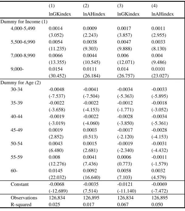
Table 1 shows the regression coe¢ cients for the income and age dummies when the dependent variables are natural logarithms of the GK and AH price indices. These two indices yield similar results. The e¤ects of age and income group dummies on the price index are stable and highly signi…cant. However, in general the values of the coe¢ cients for the GK price index are higher than those of the AH price index. As seen in Table 1, the GK price index increases with age; this is contrary to the …ndings of AH in the US. Households with higher incomes face moderately higher prices than low-income households. Based on our estimates, prices for households with income of over 9 million yen are 0.0154 points higher than prices for households in the lowest income category.

This relationship between household income and the price index plays a crucial role in creating greater price level heterogeneity in the GK price index than the AH price index. Generally, high-income families purchase more goods than low-income families. Similarly, rich families tend to face higher prices. It is clear from (6) that the GK price index is the ratio of the actual expenditure to the hypothetical expenditure. The numerator is common for both AH and GK price indices. The di¤erence between the two is in the denominator, the hypothetical expenditure. First, let us consider a commodity that is primarily purchased by rich families. Equation (8) shows that the price faced by a family with a larger GK price index is more discounted than the price faced by a family with a smaller GK price index; this which will lower the average price. Second, if the product purchased by a rich family has a signi…cantly larger share than that for a poor family, the decreasing e¤ects of the price faced by the rich family exceed the increasing e¤ects of the price faced by the poor family; again, this results in lower average prices. Thus, the average prices of commodities primarily purchased by rich families tend to be lower than their average prices in the AH price index. The lower average price results in smaller hypothetical expenditure for the rich, thereby leading to a higher GK price index for the rich. The opposite is true for poor families. Figure 2 shows the scatter plot of the two price indices, which con…rms that the di¤erence between the two indices is large for rich and poor families.

Using this GK price index, we investigate the relationship between the price level and family charac-teristics as well as observed shopping behaviors in the next section.

4

Relationship between Price and Shopping Behaviors

In this section, we decompose the contribution of the e¤ects of (1) the selection of goods and (2) the shopping behaviors on the household price index. When calculating the GK price index, we aggregate the purchase records for three months; thus, we use quarterly data. The sample period is from 2004:1Q to 2006:4Q. We compare the index for elderly households with that for young households; elderly households are de…ned as families where the wife is aged over 60, while young households are de…ned as families where the wife is younger than 30 years. We also compare the price indices for the rich (annual income is over 9 million yen) and the poor (annual income is less than 4 million yen).

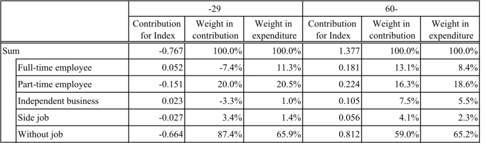
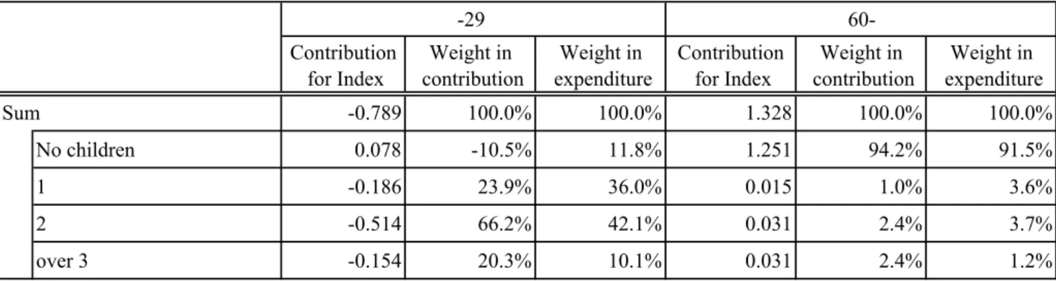
First, we check the relationship between the price index and several shopping strategies as well as observed household level characteristics. The result is moderately consistent with Abe and Shiotani (2014) who report that the price reduction mechanism based on opportunity costs of shopping provided by AH is not observed in Japan. According to Table 2, it is clear that households where the wives are full-time employees face prices that are higher than the mean price. However, high-income households with full-time homemakers whose opportunity costs are supposed to be lower than the other type of households also face higher prices. Their contribution to the index for high-income households is greater than their expenditure share. This implies that high-income households with full-time homemakers face higher prices than the other type of high-income families. Tables 4 and 5 show the relationship between the number of children and the price index. Further, they illustrate that households with young children who are supposed to be busy face lower prices than households without children. Table 4 shows that the weight of households with no children is higher for the elderly and high-income families as compared to the young or low-income families.

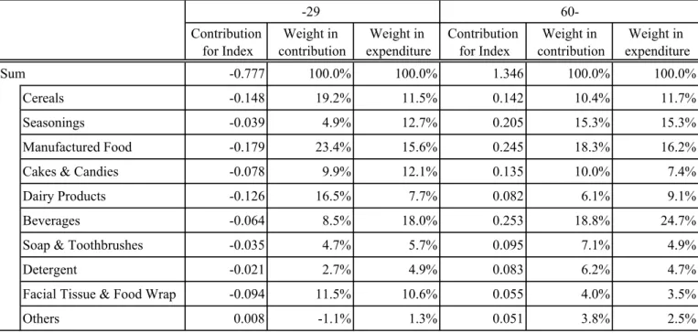
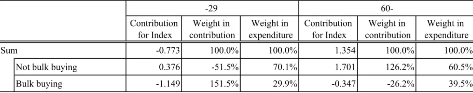
Next, we consider the e¤ect of bargain sales, which is the most important determinant of the price index according to Abe and Shiotani (2014), on the price level. Table 5 suggests that the prices of cereals, manufactured foods, and dairy products play a signi…cant role in this regard. We believe that the lower price level enjoyed by young and low-income households is primarily due to their purchase of such goods at bargain sales. Table 6 shows that price reduction is achieved only through bulk buying; that is, purchases of two or more of the same good at a time. From Table 6, we can infer that even young and low-income households that face low prices do not enjoy lower than average prices if they do not purchase two or more of the same good.

Table 7 shows that large young and low-income families can decrease their price levels through bulk buying. In contrast, the elderly and high-income households do not enjoy price reductions as the number

of family members increases.

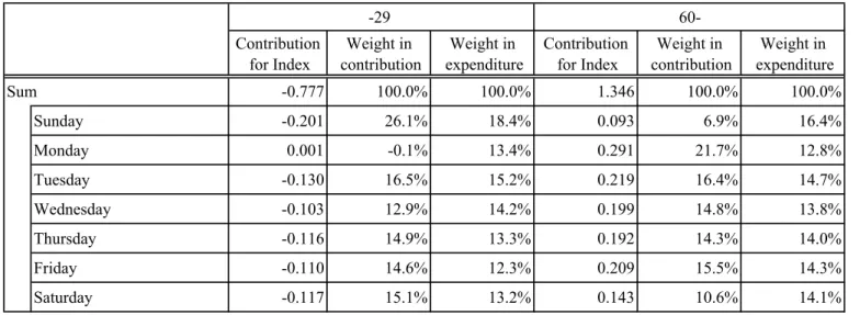
We also identify certain characteristics of the shopping behavior of the elderly that a¤ect the price index. Table 8 reports that the day of the week is an important factor that determines the price level. Shopping on Saturdays and Sundays can signi…cantly reduce the price level for the young or poor families. Over 50% of the low-income households and over 40% of the young households shop on these days. This means that the price level on weekends is lower than that on weekdays. Thus, shopping at weekend bargain sales is a crucial factor that a¤ects the heterogeneity in the household price index for the young or poor families. In contrast, the elderly buy less than the young on Sundays; this explains the di¤erence in their respective price levels to an extent.

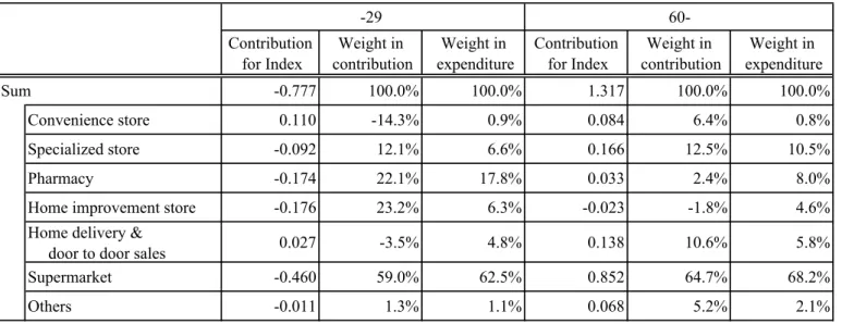
Table 9 reports the contribution of purchases at di¤erent types of stores. We observe that the elderly spend more at specialized stores and less at home improvement stores than the young; this contributes to the higher price levels among the elderly than the young. Finally, Table 10 shows that the elderly purchase more of the same goods as compared to the young. It is likely that the elderly have stronger loyalty towards some speci…c brands and may buy the same goods at non-discounted prices even if alternative goods are available at bargain prices.

5

Conclusion

This study investigates the determinants of price di¤erentials across households based on a household price index constructed using the GK method. The GK method reveals that households that buy cereals, manufactured foods, and daily products at weekend bargain sales face signi…cantly lower prices than the others. Our empirical results suggest that the number of children is an important determinant of purchases at bargain sales. Households with young children can enjoy bulk purchases at bargain sales as compared to households without children. We also …nd that certain types of shopping behaviors among the elderly such as spending more at specialized stores, spending less at home improvement stores, spending less on Sundays, and buying the same goods repeatedly contribute to their higher price levels. This paper illustrates the relationship between the household price index and several household-speci…c characteristics as well as certain patterns of shopping behaviors. In this paper, we were unable to investigate the causality in detail due to the lack of a structural model. This gap will be addressed in our future works.

6

References

References

[1] Abe, N. and Shiotani, K. (2014). Who Faces Higher Prices? An Empirical Analysis Based on Japanese Homescan Data, Asian Economic Policy Review, 9 (1), 94-115.

[2] Abe, N. and Niizeki, T. (2010). Consumption Data Based on Homescan— Comparisons with Other Consumption Data, Economic Review, 61 (3), 224-236 (in Japanese).

[3] Aguiar, M. and Hurst, E. (2007). Life-cycle Prices and Production, American Economic Review, 97 (5), 1533-1559.

[4] Baye, M., Morgan, J. and Scholten, P. (2004). Price Dispersion in the Small and in the Large: Evidence from an Internet Price Comparison Site, Journal of Industrial Economics, 52, 463-496.

[5] Geary, R.C. (1958). A Note on the Comparison of Exchange Rates and Purchasing Power Parities Between Countries, Journal of the Royal Statistical Society, 121.

[6] Haskel, J. and Wolf, H. (2001). The Law of One Price— A Case Study, Scandinavian Journal of Economics, 103, 545-558.

[7] Khamis, S.H. (1969). Neoteric Index Numbers, Bulletin of the International Statistical Institute, 43 (2), 41-42.

[8] Khamis, S.H. (1972). A New System of Index Numbers for National and International Purposes, Journal of the Royal Statistical Society, Series A.

[9] Khamis, S.H. (1984). On Aggregation Methods for International Comparisons, The Review of In-come and Wealth, 30 (2), 185-205.

[10] Meyer, S. and Schettkat, R. (2013). Price Convergence in Euroland. Evidence from Micro Data without Noise, Working Paper, Schumpeter School of Business and Economics, University of Wup-pertal.

[11] Nakamura, E. and Steinsson, J. (2008). Five Facts about Prices: A Reevaluation of Menu Cost Models, Quarterly Journal of Economics, 123(4), 1415-1464.

[12] Prasada Rao, D.S. (1985). A Walrasian Exchange Equilibrium Interpretation of the Geary-Khamis International Prices, Paper presented at the 19th General Conference of the International Associa-tion for Research in Income and Wealth, Noordwijkerhout, Netherlands, 26-31 August, 1985.

Figure 1: Distribution of Relative Price Index across Households

Note: The kernel density estimation of the price indicies defined in Section 3.

0

Figure 2: Scatter Plots of GD and AH Indices

AH

GK

AH

0.0022

0.9886

GK

0.0026

0.0031

Note: The covariance matrix is as follow, where the diagonal elements are variances, and its upper

right element is correlation.

Table 1: The Relation between Relative Price and Household Characteristics

(1)

(2)

(3)

(4)

lnGKindex

lnAHindex

lnGKindex

lnAHindex

Dummy for Income (1)

4,000-5,490

0.0014

0.0009

0.0017

0.0011

(3.052)

(2.243)

(3.857)

(2.955)

5,500-6,990

0.0054

0.0038

0.0047

0.0033

(11.235)

(9.303)

(9.888)

(8.130)

7,000-8,990

0.0066

0.0044

0.006

0.004

(13.355)

(10.545)

(12.071)

(9.486)

9,000-

0.0154

0.0111

0.014

0.0101

(30.452)

(26.184)

(26.757)

(23.027)

Dummy for Age (2)

30-34

-0.0048

-0.0041

-0.0034

-0.0033

(-7.537)

(-7.504)

(-5.363)

(-5.895)

35-39

-0.0022

-0.0022

-0.0012

-0.0018

(-3.658)

(-4.153)

(-1.771)

(-3.052)

40-44

-0.0019

-0.0022

-0.0028

-0.0034

(-3.019)

(-4.060)

(-3.850)

(-5.361)

45-49

0.0019

0.0003

-0.0017

-0.0028

(2.852)

(0.513)

(-2.120)

(-4.153)

50-54

0.0043

0.0015

-0.0019

-0.0031

(6.480)

(2.681)

(-2.340)

(-4.432)

55-59

0.008

0.0041

0.0006

-0.0011

(12.276)

(7.436)

(0.773)

(-1.579)

60-

0.0145

0.0092

0.0058

0.0032

(22.032)

(16.640)

(7.103)

(4.579)

Constant

-0.0068

-0.0035

-0.0121

-0.0069

(-12.689)

(7.514)

(-11.140)

(-7.472)

Observations

126,834

126,895

126,834

126,895

R-squared

0.025

0.017

0.067

0.050

Note:

Ordinary least squares estimates based on Japanese homescan provided by INTAGE.

The dependent variable is the Household Level AH & GK Price Index

Clustering t-statistics are in parentheses.

The data is converted to household level quarterly data.

(1) The unit is 1000yen. The base is the income below 4,000.

(2) The age of wife. The base is the dummy for below 30.

All the explanatory variables in spec (1) & (2) are shown in this table.

Spec (3)&(4) controlled for the number of family members, the age of lastchildren,

city size and prefecture .

Table 2: Contribution of Wife's job for GK index -29 60-Contribution for Index Weight in contribution Weight in expenditure Contribution for Index Weight in contribution Weight in expenditure Sum -0.767 100.0% 100.0% 1.377 100.0% 100.0% Full-time employee 0.052 -7.4% 11.3% 0.181 13.1% 8.4% Part-time employee -0.151 20.0% 20.5% 0.224 16.3% 18.6% Independent business 0.023 -3.3% 1.0% 0.105 7.5% 5.5% Side job -0.027 3.4% 1.4% 0.056 4.1% 2.3% Without job -0.664 87.4% 65.9% 0.812 59.0% 65.2%

Note: The figures are average for the sample period: 2004:1Q-2006:4Q.

-4 mil yen 9 mil

yen-Contribution for Index Weight in contribution Weight in expenditure Contribution for Index Weight in contribution Weight in expenditure Sum -0.539 100.0% 100.0% 1.169 100.0% 100.0% Full-time employee 0.077 -14.5% 8.9% 0.353 30.4% 20.8% Part-time employee -0.191 36.0% 29.9% 0.176 14.9% 33.6% Independent business -0.000 -0.1% 3.1% 0.077 6.6% 4.0% Side job -0.018 3.2% 3.2% 0.013 1.2% 1.7% Without job -0.407 75.3% 54.8% 0.549 46.9% 39.9%

Table 3: Contribution for GK index by children's age -29 60-Contribution for Index Weight in contribution Weight in expenditure Contribution for Index Weight in contribution Weight in expenditure Sum -0.789 100.0% 100.0% 1.374 100.0% 100.0% No children under 20 0.075 -10.0% 11.3% 1.279 93.3% 90.3% 0-6 -0.611 76.7% 70.3% 0.002 0.1% 1.7% 7-12 -0.038 5.0% 3.3% 0.046 3.3% 2.8% 13-19 -0.019 2.8% 1.0% 0.021 1.4% 2.6% 0-6 & 7-12 -0.191 24.9% 13.4% 0.012 0.9% 1.2% 0-6 & 13-19 0.015 -1.9% 0.4% 0.007 0.5% 0.2% 7-12 & 13-19 -0.017 2.4% 0.2% -0.003 -0.3% 1.0% 0-6, 7-12 & 13-19 - 0.0% 0.0% 0.009 0.7% 0.2%

Note: The figures are average for the sample period: 2004:1Q-2006:4Q.

-4 mil yen 9 mil

yen-Contribution for Index Weight in contribution Weight in expenditure Contribution for Index Weight in contribution Weight in expenditure Sum -0.557 100.0% 100.0% 1.192 100.0% 100.0% No children under 20 0.200 -38.0% 38.3% 0.752 63.4% 50.4% 0-6 -0.313 56.1% 22.0% 0.027 2.2% 3.9% 7-12 -0.108 19.9% 9.7% 0.057 4.8% 6.1% 13-19 -0.018 3.5% 10.9% 0.248 20.5% 26.5% 0-6 & 7-12 -0.237 43.9% 11.6% 0.028 2.4% 3.6% 0-6 & 13-19 0.005 -0.8% 0.4% 0.004 0.3% 0.4% 7-12 & 13-19 -0.071 12.7% 6.5% 0.081 6.7% 8.5% 0-6, 7-12 & 13-19 -0.015 2.8% 0.8% -0.005 -0.4% 0.6%

Table 4: Contribution of Children for GK index -29 60-Contribution for Index Weight in contribution Weight in expenditure Contribution for Index Weight in contribution Weight in expenditure Sum -0.789 100.0% 100.0% 1.328 100.0% 100.0% No children 0.078 -10.5% 11.8% 1.251 94.2% 91.5% 1 -0.186 23.9% 36.0% 0.015 1.0% 3.6% 2 -0.514 66.2% 42.1% 0.031 2.4% 3.7% over 3 -0.154 20.3% 10.1% 0.031 2.4% 1.2%

Note: The figures are average for the sample period: 2004:1Q-2006:4Q.

-4 mil yen 9 mil

yen-Contribution for Index Weight in contribution Weight in expenditure Contribution for Index Weight in contribution Weight in expenditure Sum -0.557 100.0% 100.0% 1.192 100.0% 100.0% No children 0.180 -33.0% 43.6% 0.904 76.2% 65.3% 1 -0.167 29.5% 20.5% 0.148 12.6% 17.1% 2 -0.409 72.6% 26.4% 0.099 8.3% 13.1% over 3 -0.175 31.0% 9.5% 0.035 2.9% 4.5%

Table 5: Contfibution for GK index by Goods Type -29 60-Contribution for Index Weight in contribution Weight in expenditure Contribution for Index Weight in contribution Weight in expenditure Sum -0.777 100.0% 100.0% 1.346 100.0% 100.0% Cereals -0.148 19.2% 11.5% 0.142 10.4% 11.7% Seasonings -0.039 4.9% 12.7% 0.205 15.3% 15.3% Manufactured Food -0.179 23.4% 15.6% 0.245 18.3% 16.2%

Cakes & Candies -0.078 9.9% 12.1% 0.135 10.0% 7.4%

Dairy Products -0.126 16.5% 7.7% 0.082 6.1% 9.1%

Beverages -0.064 8.5% 18.0% 0.253 18.8% 24.7%

Soap & Toothbrushes -0.035 4.7% 5.7% 0.095 7.1% 4.9%

Detergent -0.021 2.7% 4.9% 0.083 6.2% 4.7%

Facial Tissue & Food Wrap -0.094 11.5% 10.6% 0.055 4.0% 3.5%

Others 0.008 -1.1% 1.3% 0.051 3.8% 2.5%

Note: The figures are average for the sample period: 2004:1Q-2006:4Q.

-4 mil yen 9 mil

yen-Contribution for Index Weight in contribution Weight in expenditure Contribution for Index Weight in contribution Weight in expenditure Sum -0.565 100.0% 100.0% 1.172 100.0% 100.0% Cereals -0.127 22.8% 12.9% 0.139 11.8% 11.5% Seasonings -0.061 10.6% 13.7% 0.201 17.2% 13.8% Manufactured Food -0.122 21.6% 16.6% 0.221 18.8% 16.8%

Cakes & Candies -0.084 14.7% 10.2% 0.094 8.0% 8.9%

Dairy Products -0.080 14.3% 8.6% 0.065 5.5% 8.8%

Beverages -0.047 8.3% 20.6% 0.189 16.2% 22.8%

Soap & Toothbrushes -0.002 0.3% 5.1% 0.070 6.0% 5.8%

Detergent -0.001 0.2% 4.6% 0.067 5.7% 4.5%

Facial Tissue & Food Wrap -0.044 7.6% 6.0% 0.067 5.7% 4.2%

Others 0.002 -0.3% 1.7% 0.059 5.1% 2.9%

Table 6: Contribution of Bulk buying for GK index -29 60-Contribution for Index Weight in contribution Weight in expenditure Contribution for Index Weight in contribution Weight in expenditure Sum -0.773 100.0% 100.0% 1.354 100.0% 100.0%

Not bulk buying 0.376 -51.5% 70.1% 1.701 126.2% 60.5%

Bulk buying -1.149 151.5% 29.9% -0.347 -26.2% 39.5%

Note: The figures are average for the sample period: 2004:1Q-2006:4Q.

-4 mil yen 9 mil

yen-Contribution for Index Weight in contribution Weight in expenditure Contribution for Index Weight in contribution Weight in expenditure Sum -0.558 100.0% 100.0% 1.196 100.0% 100.0%

Not bulk buying 0.481 -88.7% 66.0% 1.601 134.2% 63.2%

Bulk buying -1.039 188.7% 34.0% -0.405 -34.2% 36.8%

Note: The figures are average for the sample period: 2004:1Q-2006:4Q. Table 7: Contribution for GK index by Family size

-29 60-Contribution for Index Weight in contribution Weight in expenditure Contribution for Index Weight in contribution Weight in expenditure Sum -0.777 100.0% 100.0% 1.335 100.0% 100.0% 2 0.070 -9.4% 8.8% 0.627 46.8% 50.1% 3 -0.248 32.0% 30.8% 0.451 34.0% 29.7% 4 -0.485 62.9% 39.1% 0.166 12.3% 11.2% 5 -0.122 15.5% 12.5% 0.043 3.2% 4.2% over 6 0.008 -1.0% 8.8% 0.050 3.7% 4.8%

Note: The figures are average for the sample period: 2004:1Q-2006:4Q.

-4 mil yen 9 mil

yen-Contribution for Index Weight in contribution Weight in expenditure Contribution for Index Weight in contribution Weight in expenditure Sum -0.573 100.0% 100.0% 1.187 100.0% 100.0% 2 0.134 -24.8% 27.8% 0.138 11.7% 9.9% 3 -0.021 3.2% 26.3% 0.337 28.5% 24.7% 4 -0.501 88.9% 30.8% 0.417 34.8% 36.1% 5 -0.183 32.2% 12.3% 0.159 13.4% 17.3% over 6 -0.002 0.5% 2.8% 0.137 11.5% 11.9%

Table 8: Contribution for GK index by Day of Week -29 60-Contribution for Index Weight in contribution Weight in expenditure Contribution for Index Weight in contribution Weight in expenditure Sum -0.777 100.0% 100.0% 1.346 100.0% 100.0% Sunday -0.201 26.1% 18.4% 0.093 6.9% 16.4% Monday 0.001 -0.1% 13.4% 0.291 21.7% 12.8% Tuesday -0.130 16.5% 15.2% 0.219 16.4% 14.7% Wednesday -0.103 12.9% 14.2% 0.199 14.8% 13.8% Thursday -0.116 14.9% 13.3% 0.192 14.3% 14.0% Friday -0.110 14.6% 12.3% 0.209 15.5% 14.3% Saturday -0.117 15.1% 13.2% 0.143 10.6% 14.1%

Note: The figures are average for the sample period: 2004:1Q-2006:4Q.

-4 mil yen 9 mil

yen-Contribution for Index Weight in contribution Weight in expenditure Contribution for Index Weight in contribution Weight in expenditure Sum -0.565 100.0% 100.0% 1.172 100.0% 100.0% Sunday -0.201 35.7% 17.7% 0.142 12.1% 18.5% Monday 0.035 -6.4% 12.7% 0.242 20.7% 12.7% Tuesday -0.084 15.0% 15.0% 0.178 15.2% 14.3% Wednesday -0.062 10.8% 14.0% 0.165 14.0% 13.4% Thursday -0.081 14.2% 13.4% 0.174 14.9% 13.6% Friday -0.062 10.9% 13.3% 0.156 13.2% 13.0% Saturday -0.111 19.8% 13.9% 0.116 9.8% 14.4%

Table 9: Contribution for GK index by Store type -29 60-Contribution for Index Weight in contribution Weight in expenditure Contribution for Index Weight in contribution Weight in expenditure Sum -0.777 100.0% 100.0% 1.317 100.0% 100.0% Convenience store 0.110 -14.3% 0.9% 0.084 6.4% 0.8% Specialized store -0.092 12.1% 6.6% 0.166 12.5% 10.5% Pharmacy -0.174 22.1% 17.8% 0.033 2.4% 8.0%

Home improvement store -0.176 23.2% 6.3% -0.023 -1.8% 4.6%

Home delivery &

door to door sales 0.027 -3.5% 4.8% 0.138 10.6% 5.8%

Supermarket -0.460 59.0% 62.5% 0.852 64.7% 68.2%

Others -0.011 1.3% 1.1% 0.068 5.2% 2.1%

Note: The figures are average for the sample period: 2004:1Q-2006:4Q.

-4 mil yen 9 mil

yen-Contribution for Index Weight in contribution Weight in expenditure Contribution for Index Weight in contribution Weight in expenditure Sum -0.586 100.0% 100.0% 1.141 100.0% 100.0% Convenience store 0.094 -16.2% 0.8% 0.100 8.8% 0.9% Specialized store -0.012 2.2% 6.9% 0.028 2.5% 7.5% Pharmacy -0.157 26.7% 11.5% 0.005 0.5% 9.8%

Home improvement store -0.145 25.1% 5.8% -0.053 -4.7% 5.6%

Home delivery &

door to door sales 0.041 -7.3% 5.6% 0.179 15.7% 8.5%

Supermarket -0.405 69.3% 68.0% 0.859 75.2% 66.7%

Others -0.001 0.2% 1.3% 0.023 2.0% 1.2%

Table 10: Contribution of Repeat purchasing for GK index -29 60-Contribution for Index Weight in contribution Weight in expenditure Contribution for Index Weight in contribution Weight in expenditure Sum -0.777 100.0% 100.0% 1.346 100.0% 100.0% 1 -0.552 71.4% 64.7% 0.619 46.1% 55.2% 2 -0.145 18.7% 17.0% 0.209 15.5% 17.7% 3 -0.041 5.3% 7.3% 0.135 10.1% 9.0% 4 -0.020 2.5% 3.7% 0.069 5.1% 4.8% 5 -0.006 0.8% 2.1% 0.049 3.6% 3.0% 6 -0.005 0.6% 1.3% 0.035 2.6% 2.1% 7 -0.007 0.9% 0.9% 0.028 2.0% 1.5% 8 -0.001 0.2% 0.7% 0.026 2.0% 1.1% 9 0.001 -0.2% 0.5% 0.021 1.6% 1.0% over 10 0.000 -0.1% 1.6% 0.154 11.5% 4.8%

Note: The figures are average for the sample period: 2004:1Q-2006:4Q.

-4 mil yen 9 mil

yen-Contribution for Index Weight in contribution Weight in expenditure Contribution for Index Weight in contribution Weight in expenditure Sum -0.565 100.0% 100.0% 1.165 100.0% 100.0% 1 -0.474 83.7% 59.3% 0.537 45.9% 57.5% 2 -0.118 20.9% 17.2% 0.197 17.0% 17.7% 3 -0.016 2.7% 8.2% 0.112 9.7% 8.5% 4 -0.004 0.8% 4.2% 0.069 5.9% 4.6% 5 0.006 -0.9% 2.6% 0.046 4.0% 2.8% 6 0.003 -0.5% 1.8% 0.037 3.2% 1.9% 7 0.002 -0.3% 1.3% 0.026 2.2% 1.3% 8 0.003 -0.4% 1.0% 0.023 2.0% 1.0% 9 0.001 -0.1% 0.8% 0.018 1.6% 0.8% over 10 0.033 -5.8% 3.6% 0.099 8.6% 3.9%