Experimental verification of improved
probability of detection model considering the
effect of sensor’s location on low frequency
electromagnetic monitoring signals
著者
Song Haicheng, Yusa Noritaka
journal or
publication title
International journal of applied
electromagnetics and mechanics
volume
64
number
1-4
page range
191-199
year
2020-09-03
URL
http://hdl.handle.net/10097/00130898
doi: 10.3233/JAE-209322International Journal of Applied Electromagnetics and Mechanics xx (2019) x–x 1 IOS Press
Experimental Verification of Improved
Prob-ability of Detection Model Considering the
Effect of Sensor’s Location on Low
Frequen-cy Electromagnetic Monitoring Signals
Haicheng Song
a,*, Noritaka Yusa
aaDepartment of Quantum Science and Energy Engineering, Graduate School of Engineering, Tohoku
University, 6-6-01-2, Aramaki Aza Aoba, Aoba-ku, Sendai, Miyagi, Japan
Abstract. Structural health monitoring (SHM) is a promising method for maintaining the integrity of structures. A reasonable
approach is necessary to quantify its detection uncertainty by taking into account the effect of random sensor locations on inspection signals. Recent studies of the authors proposed a model that adopts Monte Carlo simulation to numerically obtain the distribution of inspection signals influenced by random sensor locations. This model can evaluate the effect not only of multiple defect dimensions but also of the placement of sensors on the detection uncertainty. However, its effectiveness has only been confirmed using pseudo-experimental signals generated by artificial pollution. This study aims to examine the effectiveness of the proposed model in quantifying the detection uncertainty of SHM methods using the experimental signals of low frequency electromagnetic monitoring for inspecting wall thinning in pipes. The results confirm the capability of the proposed model to correctly characterize the distribution of inspection signals affected by random sensor locations and to determine the reasonable probability of detection.
Keywords:non-normal noise, probabilistic calibration, non-parametric probability density function, finite element simulation
1. Introduction
Structural health monitoring (SHM) is a promising technique for maintaining the integrity of structures with the aid of permanently installed sensors [1,2]. This method allows more frequent inspections than the traditional one-off nondestructive inspection and is able to acquire the time-varying information about the state of a target structure without disrupting the operation [3]. Nevertheless, during the inspection process, SHM is influenced by various in-situ factors that introduce noise into inspection signals and lead to detection uncertainty, namely, the errors in the decision over the presence of defects [4,5]. In practice, the quantification of the detection uncertainty of SHM systems is a major part of the reliability analyses of structures, and it demands a reasonable quantifying approach.
The probability of detection (POD) is a common metric adopted to quantify the detection uncertainty of a specific inspection method by determining the probability that a given defect is correctly detected by the method [6]. Therefore, accurately characterizing the distribution of practical inspection signals for a valid POD is essential. In the case of SHM, the placement of sensors is a decisive contributor to the detection uncertainty in addition to defect size [7-9], which arises from the dependence of signals on the distance between a sensor and a defect to be detected. Generally, the location where a defect appears in a structure is usually unknown. Therefore, the distance between a sensor and the defect is stochastic, thus causing the SHM signals to change correspondingly.
The most common method for determining POD aims to formulate a linear function with normal noise to correlate the signal amplitude with only a single variable, usually the size of a defect [10]. However, the SHM signals influenced by a random sensor location does not necessarily follow a normal distribution. Recent studies proposed several methods to determine POD by considering multiple
parameters at once [11-13], for example, the length and depth of defects, based on the idea of model-assisted POD [14] to reduce the number of experimental signals required to satisfy the statistical significance. In these methods, the simulated signals are presumed to be invariant for a specific defect profile. However, this assumption is not applicable to SHM methods because, for the same defect, the inspection signals also vary with the placement of a sensor relative to the defect.
Previous studies of the authors proposed a Monte Carlo simulation-based POD model that could correctly characterize the distribution of inspection signals affected by random sensor locations, thus quantifying the detection uncertainty of SHM methods more reasonably. The effectiveness of the proposed model has been confirmed using pseudo-experimental signals created by artificially polluting simulated signals. However, the verification based on real experimental signals has not been conducted yet.
Given the above background, this study aims to verify the effectiveness of the proposed POD model using experimental signals of low frequency electromagnetic monitoring (LFEM) [15] for inspecting wall thinning in pipes.
2. Materials and methods
Numerical simulations and experiments were performed in this work to obtain the simulated and experimental signals of LFEM to inspect pipe wall thinning. The obtained signals were subsequently analyzed by the proposed model to determine the POD to verify its effectiveness in quantifying the detection capability.
2.1. Numerical simulation
This section aims to gather the simulated LFEM signals for the POD analyses. Fig. 1 illustrates the numerical model considering the inspection of full circumferential wall thinning on the inner surface of a carbon steel pipe. The pipe was constructed to be 300 mm in length, 5.7 mm in thickness, and 45.1 mm in inner radius and was designed to be consistent with the pipe samples used in experiments. The magnetic fields were induced by an excitation coil surrounding the pipe and carrying alternative currents. The excitation coil had a square cross-section of 10 mm edge length and was mounted 45 mm away from the end of the pipe. The full circumferential wall thinning was located at the middle of the pipe and characterized by length, 𝑙, and residual thickness, 𝑡r, at its deepest position. The cross-section of the
wall thinning was shaped into a rectangle, and its fillets had a radius same as the depth (5.7-𝑡r mm) of
the wall thinning as shown in Fig. 1. Different defect profiles determined by different combinations of 𝑙
and 𝑡r were considered, and they are summarized in Table 1. As the full circumferential wall thinning
was the target of interest, the imaginary magnetic sensors were deployed only along the axial direction equidistantly with a spacing, s, and the distance between the center of the wall thinning and its nearest sensor was denoted as x, which is supposed to follow a uniform distribution x~U(-𝑠/2, 𝑠/2). The axial component of the magnetic flux density was measured along the pipe with a lift-off of 0.75 mm, so that the signals received by a sensor deployed at any location were available.
The numerical simulations to acquire the axial component of the magnetic flux density were performed using the finite element method with commercial software COMSOL Multiphysics +AC/DC module version 5.2 (Comsol Inc., USA). As the LFEM uses a weak magnetic field, the magnetic property can be supposed to be linear. The governing equation to be solved in the numerical simulations is
(𝑗𝜔𝜎-𝜔2𝜀)𝜜+∇×(𝜇-1∇×𝜜) =𝑱
𝑒 (1)
where 𝑗 is the imaginary unit, 𝜔 is the angular frequency, 𝜎 is the electric conductivity, 𝜀 is the permittivity, 𝜜 is the magnetic vector potential, 𝜇 is the magnetic permeability, and 𝑱𝑒 is the external
current density flowing in the excitation coil. The excitation frequency and current used in the simulations were 1 Hz and 20 Ampere-turn, respectively. The pipe was assumed to have a constant relative permeability of 160, an electrical conductivity of 5.2×10⁶ S/m, and a relative permittivity of 1.
The geometry was constructed in a 2D axisymmetric dimension because of the symmetry of the simulation model. The simulation domain was completely discretized into 99,391 quadratic triangular elements. The boundary condition imposed on the outmost boundary of the domain was 𝒏×𝑨=𝟶.
*
Fig. 1 Simulation model of LFEM to inspect full circumferential wall thinning, unit: mm
Fig. 2 Normalized magnetic flux density obtained in simulation and experiment when l =30 mm, tr=2 mm
Table 1 Parameters of wall thinning in numerical simulations
Parameter Value
Length of wall thinning, 𝑙 (mm) 10, 20, 30, 40, 50, 60, 70
Residual thickness, 𝑡r (mm) 1.0, 1.5, 2.0, 2.5, 3.0, 3.5, 4.0, 4.5, 5.0 2.2. Experiment
This section presents the implementation of the LFEM experiments for which a constructed experimental system [15] was adopted. Fig. 3 shows a simplified diagram of the system that is also pictured in Fig. 4. The function generator 1, WF1973 (NF Corporation, Yokohama, Japan), provided an alternating current of 1 Hz and 0.9 Vp-p, which was subsequently amplified 10 times through a power
amplifier, HSA4104 (NF Corporation, Yokohama, Japan), to an excitation coil surrounding the pipe. The excitation coil had 20 turns and was fabricated using copper wire of 1 mm diameter. The current flowing through each turn of the excitation coil was indirectly monitored using a lock-in amplifier 1, LI5640 (NF corporation, Yokohama, Japan), by measuring the voltage of a shunt resistor of 1 Ω, which was indicated to be 0.9–1.0 A. Ten magneto-impedance (MI) sensors of MI-CB-1DM A type (Aichi Micro Intelligent Corporation, Tokai, Japan) were carefully aligned and mounted on a support to compose a sensor array to measure the magnetic fields parallel to the pipe surface. The resultant distance between two neighboring MI sensors was 11 mm. Each sensor was activated in turn through relay boards, which demanded a 5 V DC voltage offered by a DC power and an AC of square wave characterized by 2,000,000/3 Hz in frequency, 5 Vp-p in amplitude, and 2.5 V in offset offered by a function generator 2,
WF 1974 (NF Corporation, Yokohama, Japan). Each sensor was kept active for 15 s to stabilize the signals. The axial component of the magnetic flux density measured by each sensor was filtered by a lock-in amplifier 2, LI5640 (NF Corporation, Yokohama, Japan), given the reference frequency. Finally, the output voltage of each MI sensor together with the excitation current was recorded by a PC using the RS-232 interface embedded in the lock-in amplifiers. The entire experimental system was controlled using Labview.
Carbon steel (STPG 370) pipe samples have the same dimensions (90A) as the numerical model presented in Figure 1. Full circumferential grooves with different profiles, which are summarized in Table 2, were artificially machined on the inner surface at the middle of the pipes to simulate wall thinning. In total, nine defective and one defect-free pipe samples were prepared.
Fig. 3 Illustration of the experimental system, unit: mm Fig. 4 Picture of experimental system
For each pipe sample, the measurement was performed at three different circumferential locations. For each circumferential location, the signals at 60 different axial positions within x∈[-55 mm, 55 mm]
were collected along the pipe surface using the sensor array.
Table 2 Parameters of the pipe samples
The amplitude of the axial component of the magnetic flux density obtained in both numerical simulation and experiment was normalized by that obtained when there was no wall thinning to obtain signal 𝐵 which is exemplified by Figure 2, as 𝐵= (Amplitude of the axial component of the magnetic flux density when a pipe has wall thinning/ 𝐼coil)/(Amplitude of the axial component of the magnetic flux
density when a pipe has no wall thinning/ 𝐼coil), where 𝐼coil is the current flowing through the coil. 𝐵 was
used in the following POD analyses.
2.3. POD analyses by the proposed model
The probability distribution of inspection signals for POD analyses should always be correctly characterized, but a proper closed-form probability density function is not always achievable. Therefore, this section explains the proposed POD model that leverages Monte Carlo simulations to numerically obtain the distribution of inspection signals affected by random sensor locations.
Because of the discrepancy between the signals measured in the actual monitoring, 𝐵mea, and the
signals obtained in the numerical simulations, 𝐵sim, this method assumes that the relationship between
two types of signal are represented in the following general form: 𝐵mea=𝑁(𝜇
1,𝜎12)(𝐵sim-min(𝐵sim)) +𝑁(𝜇2,𝜎22)+min(𝐵sim) (2)
where 𝑁(𝜇1,𝜎1) and 𝑁(𝜇2,𝜎2) are the normal distributions with means of 𝜇1 and 𝜇2 and standard
deviations of 𝜎1 and 𝜎2, respectively. The probability distribution of 𝐵mea due to wall thinning with a
certain profile was evaluated by estimating the four parameters, 𝜇1, 𝜇2, 𝜎1, and 𝜎2, using the following
procedure:
1. Assume 𝜇1, 𝜇2, 𝜎1, and 𝜎2 to be certain values.
2. Obtain 𝐵sim due to the 𝑖-th wall thinning by finite element simulation. Note that the finite element
simulation takes 𝐵sim as a function of x, and thus the distribution of 𝐵sim can be evaluated when x
follows any distribution including the uniform distribution.
3. Randomly and individually choose three values following 𝑁(𝜇1,𝜎1) and 𝑁(𝜇2,𝜎2) and the
distribution evaluated in 2 to calculate 𝐵mea according to Eq. (3). Perform this step many times to
obtain the distribution of 𝐵mea approximately.
4. Normalize and smooth the distribution obtained in 3 with the aid of kernel density estimation (KDE) [16] to obtain the probability distribution of 𝐵mea due to the 𝑖-th wall thinning, 𝑝𝑚,𝑖(𝐵).
𝑝𝑚,𝑖(𝐵)=1/(𝑛ℎ)∑𝑗𝐾(𝐵-𝐵𝑗 mea)/ℎ (3)
where 𝑛 (𝑗=1,…,𝑛) denotes the number of 𝐵mea generated in the procedure 3, ℎ is a smoothing
parameter called bandwidth, and 𝐾 is a kernel smoothing function. In this study, the Epanechnikov kernel function was adopted because of its high efficiency [16].
5. Calculate the likelihood of 𝐵𝑖exp with the assumed values of 𝜇1, 𝜇2, 𝜎1, and 𝜎2, 𝑝𝑚,𝑖(𝐵𝑖exp; 𝜇1, 𝜇2,
𝜎1, 𝜎2).
6. Perform (2)–(5) for all wall thinning under consideration, and evaluate the total likelihood by multiplying the values (or summing the log-transformed values) calculated in 5.
General derivative-free optimization algorithms enable us to find the combination of 𝜇1, 𝜇2, 𝜎1, and
𝜎2 that maximizes the total likelihood. This study used the particle swarm algorithm [17] which is a
global optimization algorithm so that the setting ofinitial values has little impacton estimation can be avoided.
POD was determined using 𝑝𝑚(𝐵) for the defects with different 𝑙 and 𝑡r given the decision threshold,
𝐵th. The confidence bounds of the POD curve were built using the basic bootstrap method [18].
3. Results and discussion
3.1. Validation of the estimated distribution
Parameter Value
Length of wall thinning, 𝑙 (mm) 10, 30, 50 Residual thickness, 𝑡r (mm) 1, 2, 3
As a precondition of a reasonable POD analysis, the validity of the proposed model to characterize the probability distribution of inspection signals affected by random sensor locations was initially examined.
The four parameters in Eq. (3), 𝜇1, 𝜇2, 𝜎1, and 𝜎2, were estimated to be 0.837, 0.090, -0.027, and 0.059,
and the corresponding confidence intervals for each estimate were [0.728, 0.924], [0.054, 0.178], [-0.099, 0.111], and [0.024, 0.1182], respectively. For this estimation, one experimental signal from each of the three measurements for each pipe sample shown in Table 2 was selected according to a randomly sampled sensor location and used as 𝐵exp. As a result, 27 observations of 𝐵exp were utilized for the
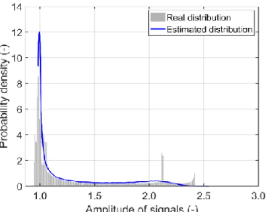
estimation and it has been examined that a larger dataset does not improve the estimation significantly. Fig. 5 compares the estimated distribution and real distribution of inspection signals when 𝑠 is assumed to be 40 mm, so that the sensor location, x, follows U(-20 mm, 20 mm). A wall thinning with 𝑙=10 mm and 𝑡r=2 mm was considered here. A total of 100,000 observations of experimental signals
sampled at random sensor locations were probabilistically evaluated to form the histogram shown in Figure 3. The same number of observations of 𝐵sim was calculated at randomly sampled x. The
observations were subsequently employed to obtain 𝐵mea according to Eq. (3) based on the estimated
values of the four parameters to acquire the distribution, which is smoothed by KDE with ℎ=0.01 and indicated by the solid line in the figure. The general agreement between the estimated distribution and real distribution indicates that the proposed model can correctly characterize the probability distribution of the inspection signals affected by random sensor locations. Some discrepancies were also observed from the comparison, and they were caused by the experimental signals obtained at different locations that were not smooth and fluctuated.
3.2. POD analyses
The effectiveness of the proposed model to determine the POD of LFEM for inspecting full circumferential wall thinning was examined. Based on the parameters estimated in section 3.1, POD analyses were implemented with a decision threshold, 𝐵th=1.15, and the inspection signals were
exempted from censoring. In Fig. 6, the consequent POD contour indicates that the detection uncertainty of LFEM is affected by both length of wall thinning and residual thickness. The lower 95% confidence bound of 0.9 POD shows that LFEM can reliably detect the full circumferential wall thinning whose profiles fall on the top-left corner. The low capability of LFEM for the defects with large residual thickness (> 4 mm) is attributed to the small amplitude of inspection signals. The detectability of defects reduces as their length decreases because of the spacing between the neighboring sensors, 𝑠=40 mm. The detection uncertainty of LFEM reflected by the generated POD contour is consistent with this result, and thus the effectiveness of the proposed model to quantify the defection uncertainty of LFEM is confirmed.
Fig. 5 Estimated probability distribution of LFEM signals affected by random sensor locations when 𝑠=40 mm, 𝑙=10
mm, 𝑡r=2 mm
Fig. 6 POD contour with the 95% confidence bounds of LFEM for inspecting full circumferential wall thinning
when 𝑠=40 mm 3.3. Effect of the sensor’s placement on POD
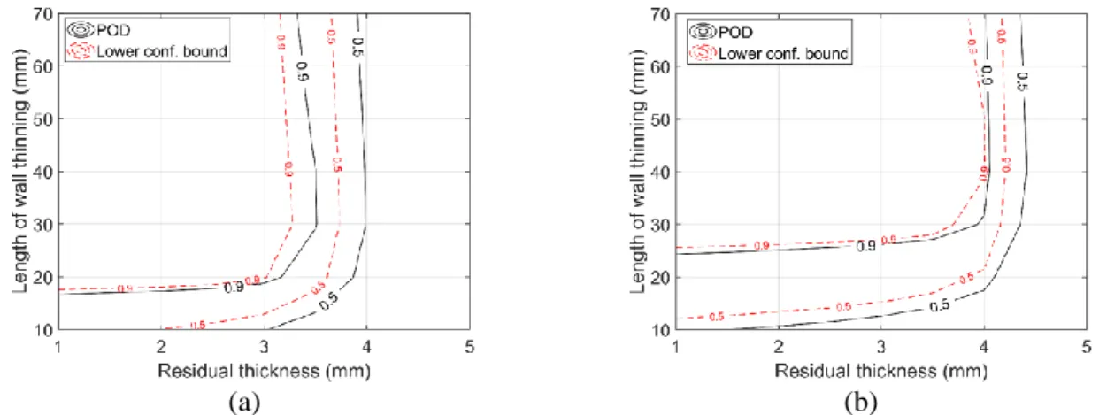
The effect of the placement of sensor, namely, the spacing between neighboring sensors, on POD was investigated. The POD analysis was implemented by the proposed model with s presumed to be 20 mm and 30 mm. Fig. 7 suggests that the defects with a shorter length can be detected with a higher probability by LFEM in comparison with the defects shown in Fig. 6, which were caused by the reduced spacing. This finding is consistent with the empirical evidence that denser sensors have a higher detection
capability with respect to the defects with a shorter length. It further confirms the validity of the proposed method to quantify the detection uncertainty of the LFEM method.
(a) (b)
Fig. 7 POD contour with the 95% confidence bounds of LFEM for inspecting full circumferential wall thinning when (a) 𝑠=20 mm and (b) s=30 mm
4. Conclusion
This study conducts experiments on LFEM for inspecting full circumferential wall thinning in carbon steel pipe samples and acquires the experimental signals affected by random sensor locations. The effectiveness of the proposed model developed on the basis of Monte Carlo simulation to quantify the detection uncertainty is examined by applying it to the POD analysis using the experimental signals. The results conclude that the proposed POD model can correctly characterize the distribution of the inspection signals affected by random sensor locations and reasonably quantify the detection uncertainty of SHM methods.
References
[1] W. Ostachowicz, R. Soman and P. Malinowski: Optimization of sensor placement for structural health monitoring: A review, Structural Health Monitoring 18 (2019), 963-988.
[2] P. Cawley, Structural health monitoring: Closing the gap between research and industrial deployment, Structural Health Monitoring 17 (2018), 1225-1244.
[3] Z. Liu and Y. Kleiner: State-of-the-art review of technologies for pipe structural health monitoring, IEEE Sensors Journal
12 (2012), 1987-1992.
[4] J. F. C. Markmiller and F. K. Chang: Sensor network optimization for a passive sensing impact detection technique. Structural Health Monitoring 9 (2010), 25-39.
[5] V. Janapati, F. Kopsaftopoulos, F. Li, S. J. Lee and F. Chang: Damage detection sensitivity characterization of acousto-ultrasound-based structural health monitoring techniques, Structural Health Monitoring 15 (2016), 143-161.
[6] L. Gandossi and K. Simola: Derivation and use of probability of detection curves in the nuclear industry, Insight-Non-Destructive Testing and Condition Monitoring 12 (2010), 657-663.
[7] Y. H. Teo, W. K. Chiu, F. K. Chang and N. Rajic: Optimal placement of sensors for sub-surface fatigue crack monitoring. Theoretical and Applied Fracture Mechanics 25 (2009), 40-49.
[8] M. Azarbayejani, A. I. El-Osery, K. K. Choi and M. M. Reda Taha: A probabilistic approach for optimal sensor allocation in structural health monitoring, Smart Materials and Structures 17 (2008), 055019.
[9] J. F. C. Markmiller and F. K. Chang: Sensor network optimization for a passive sensing impact detection technique, Structural Health Monitoring 9 (2010), 25-39.
[10] A. P. Berens: NDE reliability data analysis, ASM Handbook, 17 (1989), 689-701.
[11] N. Yusa and J. S. Knopp: Evaluation of probability of detection (POD) studies with multiple explanatory variables, Journal of Nuclear Science and Technology 53 (2016), 574-579.
[12] N. Yusa, W. Chen and H. Hashizume: Demonstration of probability of detection taking consideration of both the length and the depth of a flaw explicitly, NDT & E International 81 (2016), 1-8.
[13] M. Pavlović, K. Takahashi and C. Müller: Probability of detection as a function of multiple influencing parameters, Insight-Non-Destructive Testing and Condition Monitoring 54 (2012), 606-611.
[14] R. B. Thompson: A Unified Approach to the Model‐Assisted Determination of Probability of Detection, AIP Conference Proceedings 975 (2008), 1685-1692.
[15] H. Song, N. Yusa and H. Hashizume: Low Frequency Electromagnetic Testing for Evaluating Wall Thinning in Carbon Steel Pipe, Materials Transactions 59 (2018), 1348-1353.
[16] Y. C. Chen: A tutorial on kernel density estimation and recent advances, Biostatistics & Epidemiology 1 (2017), 161-187. [17] J. F. Schutte, J. A. Reinbolt, B. J. Fregly, R. T. Haftka and A. D. George: Parallel global optimization with the particle
swarm algorithm, International journal for numerical methods in engineering 61 (2004), 2296-2315.
受理通知メールコピー(国際会議 ISEM2019 の Full Paper として International Journal of Applied Electromagnetics and Mechanics 誌に投稿のため ISEM2019 通知は事務局より)
From: <[email protected]> Date: Sun, Apr 5, 2020 at 9:13 PM Subject: Manuscript 19-41-R Decision To: <[email protected]>
Dear Dr. Song:
Your manuscript (19-41-R) has been accepted in ISEM2019. A proof of your manuscript will arrive within the next weeks. Thank you for your excellent contribution, and we look forward to receiving further submissions from you in the future.
Sincerely, Jinhao QIU ISEM2019
To obtain reviews and confirm receipt of this message, please visit: https://msTracker.com/reviews.php?id=145100&aid=262638