東北大学機関リポジトリTOUR

(1)

Reconfiguration of Subgraphs Satisfying

Specific Properties

著者

水田遥河

学位授与機関

Tohoku University

学位授与番号

11301甲第19346号

URL

http://hdl.handle.net/10097/00130236

(2)

Reconfiguration of Subgraphs Satisfying

Specific Properties

by

Haruka Mizuta

Submitted to

Department of System Information Sciences

in partial fulfillment of the requirements for the degree of

Doctor of Philosophy (Information Sciences)

Graduate School of Information Sciences

Tohoku University, Japan

(3)

(4)

i

Acknowledgements

First of all, I would like to express the deepest appreciation to my supervisor, Pro-fessor Xiao Zhou. He always gave me valuable guidances and comments that made my research more sophisticate, and helpful suggestion for my research direction. He also provided a pleasant environment for my research in the laboratory. Without his encouragement, this thesis would not have been materialized.

I would like to express very special thanks to my thesis advisor, Associate Professor Takehiro Ito. He always helped me on the presentations in conferences and on the writing style of my papers. He also gave me a lot of opportunities of cooperative research with researchers in other universities. All experience in these opportunities helped on my growing as a researcher.

I would also like to thank Associate Professor Akira Suzuki for his helpful sug-gestions and guidance. He took a lot of time to discuss with me, and I learned from him how to proceed with the research. I am also very grateful to his support in my laboratory life.

I would also like to show my special thanks to the other members of my graduate committee, Professor Ayumi Shinohara and Professor Takuo Suganuma for their insightful suggestions and comments.

I am deeply grateful to Tatsuhiko Hatanaka. He had discussion with me many times, and gave me valuable comments and suggestions.

(5)

ii

My heartfelt gratitude goes to Professor Naomi Nishimura and her students Ben-jamin Moore, Vijay Subramanya and Krishna Vaidyanathan at University of Water-loo, and Research Associate Tesshu Hanaka at Chuo University. Without valuable discussions with them, this thesis would not have been completed.

Also, I would like to oﬀer my special thanks to all members of the project of Development of Algorithmic Techniques for Combinatorial Reconfiguration (DAT-CORE project). I really enjoyed the discussions with them, and they have greatly influenced me.

Finally, I would like to acknowledge with sincere thanks the all-out cooperation and services rendered by the members of Algorithm Theory Laboratory for many things.

(6)

iii

Abstract

Combinatorial reconfiguration is one of the well-studied topics in the field of theoret-ical computer science, which was introduced by Ito et al. in 2008. This topic deals with a “dynamic transformation” of feasible solutions; more specifically, in a (combi-natorial) reconfiguration problem, we wish to find a step-by-step transformation be-tween feasible solutions such that all intermediate ones in the transformation are also feasible solutions. In this thesis, we mainly studied reconfiguration problems from the following two viewpoints. The first one is to develop polynomial-time algorithms for reconfiguration problems whose feasible solutions are connected subgraphs. From the previous studies, it is known to be hard to construct an eﬃcient algorithm solv-ing a reconfiguration problem if its feasible solutions are connected subgraphs. We focused on several graph properties which require the connectivity, and analyzed the computational complexity of reconfiguration problems of subgraphs satisfying the property. Throughout this analysis, we developed many polynomial-time algo-rithms solving the reconfiguration problems with connected subgraphs. The second one is to introduce a new variant of reconfiguration problems, called “optimization variant,” in which we do not need to specify a target solution and are asked for a desirable solution that is reachable from an initial solution. As the first example of this variant, we applied this variant to the reconfiguration problem of indepen-dent sets which is one of the most well-studied reconfiguration problems. We then analyzed its polynomial-time solvability and parameterized complexity.

(7)

iv

List of Figures

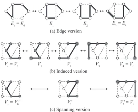
1.1 An example of a transformation from feasible supplies (a) to (d), where square vertices correspond to power stations, circle vertices to customers, lines to candidates for each customer, and black solid lines to feasible supply. . . . 2 1.2 Reconfiguration sequences in the three versions under TJ with the

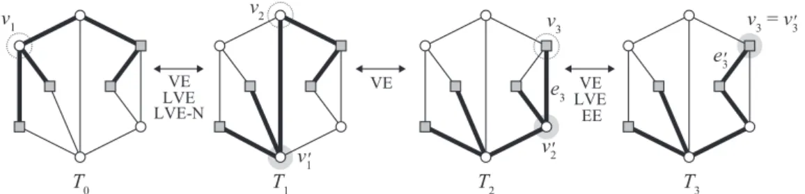
property “a graph is a path,” where the subgraphs satisfying the property by thick lines and in (b) and (c), vertices forming solutions are depicted by gray circles. . . . 6 1.3 A sequence of Steiner trees, where the terminals are depicted by gray

squares, non-terminals by white circles, the edges in Steiner trees by thick lines. . . . 8 1.4 Our results for the reconfiguration problem of Steiner trees under

VE, LVE and EE, where each square corresponds to a graph class, and

A→ B means that A contains B as a subclass. . . 12

1.5 Our results for the reconfiguration problem of minimum Steiner trees under LVE-N, where each square corresponds to a graph class, and

A→ B means that A contains B as a subclass. . . 13

1.6 A sequence⟨I0, I1, I2, I3⟩ of independent sets under TAR for the lower

bound l = 1, where the vertices in independent sets are colored with black. . . . 14

(11)

viii

1.7 _{Our results for Opt-ISR, where each square corresponds to a graph} class, and A→ B means that A contains B as a subclass. . . 16 3.1 Reduction to the edge version under TJ for the property “a graph is

a path.” . . . 27 3.2 Reconfiguration sequence ⟨E0, E1, E2⟩ in the edge version under TJ

with the property “a graph is a tree.” . . . 31 3.3 Illustration for the proof of Theorem 3.11. . . 38 3.4 Reduction for the property “a graph is an (i, j)-biclique” for any fixed

i≥ 1. . . 39

3.5 Reduction for the property “a graph is a (k, k)-biclique.” . . . 41 3.6 Reduction for the property “a graph has diameter at most two.” The

vertices of Vsin G and of Vs′ in G′ are depicted by gray vertices, where

rx = r2. . . . 46

4.1 (a) An input graph G′ of MVCR with a minimum vertex cover C′, where the vertices in C′ are depicted by gray vertices, and (b) its corresponding planar graph G of the auxiliary problem together with the minimum Steiner set to C′, where face-terminals are depicted by triangles, edge-terminals by squares, and connected subgraph corre-sponding to the minimum Steiner set by thick lines. . . 54 4.2 (a) The dual graph of the graph G in Figure 4.1(a) with a path P′

between w′_p and w′_q depicted by thick lines, and (b) a walk between

(12)

ix

4.3 (a) An example of an input graph G′ of MVCR with a vertex cover C′ represented by colored vertices, and (b) its corresponding split graph

G of the auxiliary problem with the Steiner set corresponding to C′, where terminals are depicted by squares, and the connected subgraph corresponding to the Steiner set by thick lines. . . 57 4.4 Illustration for the proof of Proposition 1. . . . 59

4.5 Illustration for the proof of Lemma 4.5. . . 61 4.6 Illustration for the proof of Lemma 4.6, where the intervals in Fp are

depicted by thick gray lines and those in Fq by thin black lines. . . . 63 4.7 (a) An example of a cycle in H with P depicted by thick lines, and

(b) the corresponding reconfiguration sequence ⟨Tj = T3′, T2′, T1′, T0′ =

Tj+1⟩ under LVE between Tj and Tj+1. . . . 72 4.8 An example of Lemma 4.19, where (a) a subtree T′, and (b) G′

cor-responding to T′ and an embedding φ such that φ(x) = u. . . 80 4.9 An example of Lemma 4.20, where (a) T with a branching node x,

and (b) G with subgraphs G1, G2, and G3. . . 81

4.10 The subtree T depicted by thick lines is a minimum Steiner tree. However, the subpath on T between s and x is not a shortest path in the underlying graph. . . 82 4.11 An example of Line 3 in the algorithm, where (a) a branching node

x with its close nodes y1, y2, and y3, and (b) a vertex u we look for

in Line 3. . . . 83

4.12 An example of Line 5 in the algorithm, where (a) a node x with close nodes y and z such that the unique path y and z contains x, and (b) a vertex u we look for in Line 5. . . 84

(13)

x

4.13 (a) A sequence of induced subgraphs G[Fi] obtained by a Steiner set sequenceF = ⟨F0, F1, . . . , Fℓ⟩, and (b) its corresponding reconfigura-tion sequence. . . 100 5.1 (a) Graph G′ and its independent set I_r′ _{for MISR, and (b) the}

cor-responding graph G for Opt-ISR, where newly added edges are de-picted by thick dotted lines. . . 104 5.2 Illustration for Lemma 5.8, where two vertices b′_i, b′_j ∈ S \ C are

depicted by squares. By the definition of a sunflower, all vertices v adjacent to both b′_i and b′_j must be contained in C = NG[b′i]∩ NG[b′j]. 114

(14)

1

Chapter 1 Introduction

1.1 Combinatorial reconfiguration

Combinatorial reconfiguration [18] is one of the well-studied topics in the field

of theoretical computer science. (See surveys [17, 29].) This topic deals with a “dynamic transformation” of feasible states; more specifically, we wish to find a step-by-step transformation between feasible states such that all intermediate ones in the transformation are also feasible states. Combinatorial reconfiguration has several applications such as dynamic puzzle games (e.g. 15 puzzle [20]) and a transition of system states which deliver continuous service.

As an example in the later application, consider a power supply system [18] in which power stations with fixed capacity provide power to customers with fixed demand. (See Figure 1.1.) In this system, each customer has several power stations as candidates of supply source, and is indeed provided power from exactly one of the candidates. Then it is necessary that for each power station, the sum of demands of customers to which the station provides power is at most the capacity of the station; such a supply is called a “feasible supply.” As an example, Figure 1.1 illustrates four feasible supplies (a), (b), (c) and (d). We now consider a dynamic transformation of states of the power supply system; we wish to transform a current feasible supply into another feasible supply. To minimize interruption, this transformation needs to be done by repeatedly switching the source power station of a single customer at a time, while keeping feasibility during the transformation. For example, Figure 1.1 illustrates a transformation between the feasible supplies (a) and (d).

(15)

2 Chapter 1 Introduction 100 80 80 50 20 60 30 100 80 80 50 20 60 30 100 80 80 50 20 60 30 100 80 80 50 20 60 30 (a) (b) (c) (d)

Figure 1.1: An example of a transformation from feasible supplies (a) to (d), where square vertices correspond to power stations, circle vertices to customers, lines to candidates for each customer, and black solid lines to feasible supply.

In general, a transformation of system states consists of the following framework: We need to transform a feasible state into another feasible state by repeatedly apply-ing a prescribed change operation at a time. In 2008, Ito et al. [18] formulated such a dynamic situation as combinatorial reconfiguration. Generally, a (combinatorial)

reconfiguration problem studies the reachability/connectivity of feasible solutions in

a “solution space.” A solution space is defined as a graph such that the vertex set corresponds to a set of all feasible states, and there is an edge between two feasible states that are “adjacent,” according to a prescribed adjacency relation. Feasible states in a solution space are often defined as feasible solutions of an instance of a tra-ditional search problem, and hence feasible states are often called feasible solutions. Then, a reachability variant of a reconfiguration problem asks to determine whether or not there is a path in a solution space from a specified solution (called an initial

solution) to another specified solution (called a target solution). We call such a path

a reconfiguration sequence between the initial and target solutions, and if it exists, we say that the initial and target solutions are reachable. There is another variant of reconfiguration problems, called a connectivity variant. This variant asks to deter-mine whether a reconfiguration graph is connected or not, that is, any two feasible solutions are reachable or not. Since the 2000s, several reconfiguration problems are introduced based on traditional search problems and studied its computational complexity; for example, vertex coloring [6, 9, 35], vertex cover [18, 25], in-dependent set [18, 22], matching [18], shortest path [4, 5, 21], clique [19],

(16)

1.2 Reconfiguration of (connected) subgraphs 3

induced tree [34], and Hamiltonian cycle [33].

In this thesis, we mainly studied reconfiguration problems from the following two viewpoints. The first one is to develop eﬃcient (polynomial-time) algorithms solving reconfiguration problems whose feasible solutions are connected subgraphs. The second one is to introduce a new variant of reconfiguration problems called “optimization variant,” in which we do not need to specify a target solution and are asked for a desirable solution that is reachable from an initial solution.

1.2 Reconfiguration of (connected) subgraphs

In previous studies, many reconfiguration problems take subgraphs as its feasible solutions, and many eﬃcient algorithms were developed for these problems. How-ever, there are few algorithms for reconfiguration problems whose feasible solutions are “connected” subgraphs. We thus see that it is hard to develop an algorithm for reconfiguration problem with connected subgraphs.

In the field of search problems, it is also known that developing an algorithm for problem with connected subgraphs are quite hard. For example, in 1983, Baker [2] gave a general approach for deriving a polynomial-time approximation schemes on planar graphs. His method can be applied for many search problems, however, it sometimes doesn’t work for problems with connectivity. Then, in 2007 (after more than twenty years), Borradaile et al. [7] provided a new technique which deriver a polynomial-time approximation schemes on planar graphs for a problem with connectivity. Similar breakthrough was also occurred in the area of parameterized complexity. It had been believed until very recently that there is no algorithm in time faster than O∗(twtw) with respect to the treewidth tw of an input graph for problems with connectivity However, in 2011, Cygan et al. [11] gave an algorithm method which solves a problem with connectivity in time O∗(ctw_{) for some constant}

(17)

4 Chapter 1 Introduction

1.2.1 Our problems

In Chapter 3 and 4, we aim to develop eﬃcient (polynomial-time) algorithms for reconfiguration problems that take connected subgraphs as its feasible solutions. We use the term subgraph reconfiguration to describe a family of reconfiguration problems with (not necessary connected) subgraphs. Each of the individual problems in the family can be defined by specifying a solution space, that is, specifying the vertex set (feasible solutions) and the edge set (adjacency relation) of the solution space. In particular, feasible solutions are defined in terms of a graph structure property Π which subgraphs must satisfy; for example, “a graph is a tree,” “a graph is edgeless (an independent set),” and so on. In this thesis, we study the following two problems that belong to subgraph reconfiguration.

Reconfiguration of fundamental graphs.

In the first problem, we focus on six fundamental graph properties as a property Π; path, cycle, tree, clique, bi-clique, and diameter-two. For each property Π, we consider a reconfiguration problem whose solution space is defined as follows.

Feasible solutions (i.e., vertices in the solution space) are defined as subgraphs satisfying Π. By the choice of how to represent the subgraphs, we introduce three versions; in each version, subgraphs are represented by vertex subsets or edge sub-sets, as follows.

- Edge version: An edge subset induces a subgraph that satisfies Π. - Induced version: A vertex subset induces a subgraph that satisfies Π.

- Spanning version: A vertex subset induces a subgraph that contains at least

one spanning subgraph satisfying Π.

As an example, Figure 1.2 illustrates several feasible solutions in each version with the property “a graph is a path.” In this figure, V₁′ is feasible in the spanning

(18)

version, while is not feasible in the induced version, because it does not induce a path. As can be seen by this simple example, in the spanning variant, we need to pay attention to the additional complexity of finding a spanning subgraph and the complications resulting from the fact that the subgraph induced by the vertex subset may contain more than one spanning subgraph which satisfies Π.

We then define an adjacency relation (i.e., edges in the solution space). Since we represent a feasible solution by a set of vertices (or edges) in any version, we can consider that tokens are placed on each vertex (resp., edge) in the feasible solution. Then, we mainly deal with the following two well-known adjacency relation [19, 22]:

- Token-jumping (TJ, for short): We say that two solutions are adjacent under

TJ if one can be obtained from the other one by moving a single token to any other vertex (edge) in a given graph.

- Token-sliding (TS, for short): We say that two solutions are adjacent under

TS if one can be obtained from the other one by moving a single token to an adjacent vertex (adjacent edge, that is sharing a common vertex).

As an example, Figure 1.2 shows reconfiguration sequences in each version under TJ. (We note that in Chapter 5, we consider another well-studied adjacency relation, called token-addition-and-removal (TAR, for short) [18, 19, 22], where we can add or remove a single token at a time.)

In Chapter 3, we study the reachability variant of reconfiguration problems whose solution spaces are defined above, that is, we are given two feasible solutions and asked to determine whether or not there is a path between them in the solution space.

(19)

V

s = V0 V1 V2 V3 V4 = Vt

(a) Edge version

(b) Induced version V s = V0 V1 V2 = Vt (c) Spanning version

ʹ

E s = E0 E1 E2 E3 = Et

Figure 1.2: Reconfiguration sequences in the three versions under TJ with the prop-erty “a graph is a path,” where the subgraphs satisfying the propprop-erty by thick lines and in (b) and (c), vertices forming solutions are depicted by gray circles.

Reconfiguration of Steiner trees.

In the second problem, we focus on the concept of “Steiner tree” as a property Π; note that in the two breakthrough papers for search problems mentioned at the beginning of this section, the search problem of Steiner trees is considered as a typical problem with connectivity. For an unweighted graph G and a vertex subset

S ⊆ V (G), a Steiner tree of G for S is a subtree of G which includes all vertices

in S; each vertex in S is called a terminal. For example, Figure 1.3 illustrates four Steiner trees. Then the second problem takes Steiner trees as a property Π. More specifically, we consider reconfiguration problems whose solution spaces are defined, as follows.

Feasible solutions (i.e., vertices in the solution space) are defined as all Steiner trees of a given graph. Note that unlike the previous problem, a feasible solution is a graph itself, not a vertex subset or an edge subset.

(20)

four adjacency relations:

- Vertex exchange (VE, for short): We say that two Steiner trees T and T′ of G for S are adjacent under VE if there exist two vertices v ∈ V (T ) and v′ ∈ V (T′) such that their removal results in the common vertex subset; it is equivalent to the condition |V (T ) \ V (T′)| = |V (T′)\ V (T )| ≤ 1.

- Local vertex exchange (LVE, for short): We say that two Steiner trees T and

T′ of G for S are adjacent under LVE if there exist two vertices v ∈ V (T ) and

v′ ∈ V (T′) such that their removal results in the common subgraph of T and T′.

- Local vertex exchange without changing neighbors (LVE-N for short):

We say that two Steiner trees T and T′ of G for S are adjacent under LVE-N if there exist two vertices v ∈ V (T ) and v′ ∈ V (T′) such that (a) their removal results in the common subgraph of T and T′, and (b) the neighborhood of v in

T is equal to that of v′ in T′.

- Edge exchange (EE, for short): We say that two Steiner trees T and T′ of G

for S are adjacent under EE if there exist two edges e ∈ E(T ) and e′ ∈ E(T′) such that their removal results in the common edge subset (and hence, common subgraph of T and T′); it is equivalent to the condition|E(T )\E(T′)| = |E(T′)\

E(T )| ≤ 1.

As an example, in Figure 1.3, any two consecutive Steiner trees are adjacent under VE. However, considering LVE, T1 and T2 are not adjacent because removing v2

from T1 and v′2 from T3 result in the diﬀerent subgraphs. Under LVE-N, only two

Steiner trees T0 and T1 are adjacent, because v1 in T0 has the same neighborhood

with v₁′ in T1. Under EE, only two Steiner trees T2 and T3 are adjacent, because the

subgraph of T2 obtained by removing e3 is equal to the subgraph of T3 obtained by

removing e′₃. It should be note that v and v′ can be the same vertex in VE, LVE, and LVE-N, and e and e′ can be the same edge in EE. (See T2 and T3 under VE or LVE in

(21)

8 Chapter 1 Introduction T 0 T1 v 1 v 1 v 2 v 3 = v3 T 2 T3 ′ v 2 ′ ′ ′ v 3 e 3 e 3 LVE LVE VE VE EE VE LVE-N

Figure 1.3: A sequence of Steiner trees, where the terminals are depicted by gray squares, non-terminals by white circles, the edges in Steiner trees by thick lines.

In Chapter 4, we study the reachability variant of reconfiguration problems whose feasible solutions are Steiner trees, that is we are given two Steiner trees, and asked to determine whether or not there is a path between them in the solution space defined above.

1.2.2 Known and related results

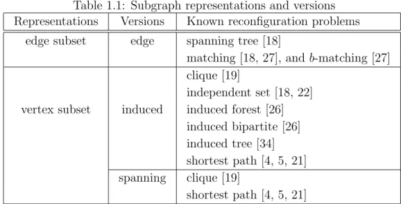
Although there has been previous work that can be categorized as subgraph re-configuration, most of the related results appear under the name of the property Π under consideration. Accordingly, we can view reconfiguration of independent sets [18, 22] as the induced version of subgraph reconfiguration such that the property Π is “a graph is edgeless.” Other examples can be found in Table 1.1. We here explain only known results which are directly related to our contributions.

Reconfiguration of cliques can be seen as both the spanning and the induced ver-sion; the problem is PSPACE-complete under any adjacency relation, even when restricted to perfect graphs [19]. Indeed, for this problem, the rules TAR, TJ, and TS have all been shown to be equivalent from the viewpoint of polynomial-time solv-ability. It is also known that reconfiguration of cliques can be solved in polynomial time for several well-known graph classes [19].

Wasa et al. [34] considered the induced version under the TJ and TS rules with the property Π being “a graph is a tree.” They showed that this version under each of the TJ and TS rules is PSPACE-complete, and is also W[1]-hard when parameterized

(22)

Table 1.1: Subgraph representations and versions Representations Versions Known reconfiguration problems

edge subset edge spanning tree [18]

matching [18, 27], and b-matching [27] clique [19]

independent set [18, 22] vertex subset induced induced forest [26]

induced bipartite [26] induced tree [34] shortest path [4, 5, 21] spanning clique [19]

shortest path [4, 5, 21]

by both the size of a solution and the length of a reconfiguration sequence. They also gave a fixed-parameter algorithm when parameterized by both the size of a solution and the maximum degree of an input graph, under both the TJ and TS rules. In closely related work, Mouawad et al. [26] considered the induced versions under the TAR rule with the properties Π being either “a graph is a forest” or “a graph is bipartite.” They showed that these versions are W[1]-hard when parameterized by the size of a solution plus the length of a reconfiguration sequence.

Bonsma [4, 5] studied the induced and spanning versions under the TJ rule with the property Π being “a graph is a shortest st-path;” note that these two versions are equivalent for this property because of the shortestness of paths. He showed that the problem is PSPACE-complete even for bipartite graphs [4], while polynomial-time solvable for chordal graphs [4], craw-free graphs [4], and planar graphs [5]. Wrochna [35] also studied this problem and showed that it is PSPACE-complete even for bounded bandwidth graphs. Although the hardness results for bipartite graphs and bounded bandwidth graphs has been shown independently, a simple observation implies that this problem remains PSPACE-complete even for bipartite graphs with bounded bandwidth graph. We should note that this problem is special case of the reconfiguration problem of Steiner trees under three adjacency relations,

(23)

VE, LVE, and LVE-N; the reconfiguration problem of Steiner trees is equivalent to that of shortest st-paths if the number of terminals are exactly two and given two Steiner trees have minimum number of edges. Therefore, the hardness results for the reconfiguration problem of shortest st-paths also hold for that of Steiner trees.

1.2.3 Our contribution

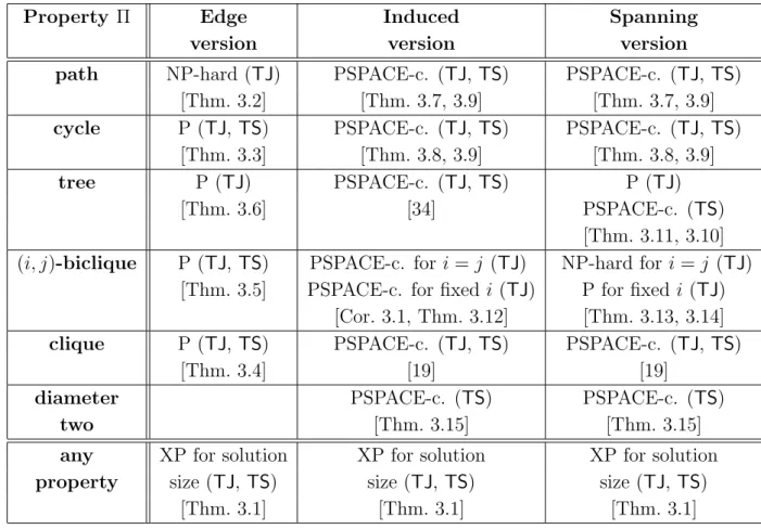
We first describe our results for the reconfiguration problems with six fundamental graph properties. (Our results are summarized in Table 1.2, together with known results, where an (i, j)-biclique is a complete bipartite graph with the bipartition of

i vertices and j vertices.) As mentioned above, since we consider the TJ and TS

rules, it suﬃces to deal with subgraphs having the same number of vertices or edges. Subgraphs of the same size may be isomorphic for certain properties Π, such as “a graph is a path” and “a graph is a clique,” because there is only one choice of a path or a clique of a particular size. On the other hand, for the property “a graph is a tree,” there are several choices of trees of a particular size. (We will show an example in Section 3.3 with Figure 3.2.)

As shown in Table 1.2, we systematically clarify the complexity of reconfiguration problems for the six fundamental graph properties. In particular, we show that the edge version under TJ is computationally intractable for the property “a graph is a path” but tractable for the property “a graph is a tree.” This implies that the computational (in)tractability for various properties Π does not follow directly from the inclusion relationships among the graph classes specified in the properties; one possible explanation is that the path property implies a specific graph, whereas the tree property allows several choices of trees, making the problem easier. To the best of the author’s knowledge, entries missing from Table 1.2 (such as the examination of several properties under TS) remain open problems.

(24)

Table 1.2: Previous and new results

Property Π Edge Induced Spanning

version version version

path NP-hard (TJ) PSPACE-c. (TJ, TS) PSPACE-c. (TJ, TS) [Thm. 3.2] [Thm. 3.7, 3.9] [Thm. 3.7, 3.9]

cycle P (TJ, TS) PSPACE-c. (TJ, TS) PSPACE-c. (TJ, TS)

[Thm. 3.3] [Thm. 3.8, 3.9] [Thm. 3.8, 3.9]

tree P (TJ) PSPACE-c. (TJ, TS) P (TJ) [Thm. 3.6] [34] PSPACE-c. (TS)

[Thm. 3.11, 3.10] (i, j)-biclique P (TJ, TS) PSPACE-c. for i = j (TJ) NP-hard for i = j (TJ)

[Thm. 3.5] PSPACE-c. for fixed i (TJ) P for fixed i (TJ) [Cor. 3.1, Thm. 3.12] [Thm. 3.13, 3.14]

clique P (TJ, TS) PSPACE-c. (TJ, TS) PSPACE-c. (TJ, TS)

[Thm. 3.4] [19] [19]

diameter PSPACE-c. (TS) PSPACE-c. (TS)

two [Thm. 3.15] [Thm. 3.15]

any XP for solution XP for solution XP for solution

property size (TJ, TS) size (TJ, TS) size (TJ, TS)

[Thm. 3.1] [Thm. 3.1] [Thm. 3.1]

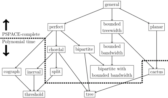
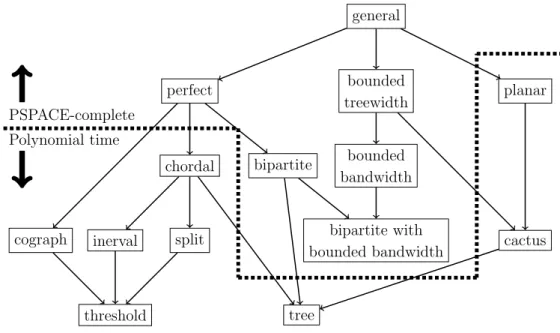
we mentioned, the problems under VE, LVE and LVE-N are generalizations of the reconfiguration problem of shortest paths. Following the problem of shortest st-paths, we studied the problems of Steiner trees with respect to graph classes. We first showed that the problem under each of VE, LVE and EE is PSPACE-complete even for split graphs and planar graphs, while polynomial-time solvable for cographs, interval graphs and cactus graphs. (See Figure 1.4.) We further studied the special case where given two Steiner trees have minimum number of edges. Then we showed that the problem under EE is polynomial-time solvable for any graph, while that under VE and LVE has the same computational complexity with the general (not necessary minimum) case. For this special case, we also studied under LVE-N. Specifically, we showed that the reconfiguration problem of minimum Steiner trees under LVE-N is polynomial-time solvable for chordal graphs and planar graphs. (See Figure 1.5.)

(25)

general

perfect bounded

treewidth planar

chordal bipartite bounded

bandwidth

cograph inerval split bipartite with

bounded bandwidth cactus

threshold tree

PSPACE-complete Polynomial time

Figure 1.4: Our results for the reconfiguration problem of Steiner trees under VE, LVE and EE, where each square corresponds to a graph class, and A → B means that A contains B as a subclass.

By considering several properties with connectivity, we proposed several polynomial-time algorithms solving reconfiguration problems whose feasible solu-tions are connected subgraphs.

1.3 New variant of reconfiguration problems

In the reachability variant of reconfiguration problems, we need to specify a tar-get solution. However, there may exist (possibly, exponentially many) desirable solutions (candidates of a target solution); even if we cannot reach a given target solution from the initial solution, there may exist another desirable solution which is reachable.

1.3.1 Our problem

In this thesis, we propose a new variant of reconfiguration problems in which we are only given an initial solution and asked to find more desirable solution that is reachable from the initial solution. We call this variant the optimization variant. As

(26)

1.3 New variant of reconfiguration problems 13

general

perfect bounded

treewidth planar

chordal bipartite bounded

bandwidth

cograph inerval split bipartite with

bounded bandwidth cactus

threshold tree

PSPACE-complete Polynomial time

Figure 1.5: Our results for the reconfiguration problem of minimum Steiner trees under LVE-N, where each square corresponds to a graph class, and A → B means that A contains B as a subclass.

the first example of this variant, we consider independent set reconfiguration (the reconfiguration problem of independent sets) under TAR rule [18, 22] because it is one of the most well-studied reconfiguration problems.

For a graph G, an independent set of G is a vertex subset I ⊆ V (G) in which no two vertices are adjacent. Then, independent set reconfiguration is a re-configuration problem whose rere-configuration graph is defined as follows: The vertex set is a set of all independent sets whose cardinalities are at least a given number l, and two independent sets are adjacent if the size of symmetric diﬀerence of them is exactly one; this adjacency relation is one of the well-studied relation,

calledtokne-addtion-and-removal (TAR, for short) [18, 19, 22]. Figure 1.6 illustrates an example

of reconfiguration sequence between two independent sets I0 and I3 under TAR for

the lower bound l = 1.

Then we consider the optimization variant of independent set reconfigu-ration; for simple notation, we denoted by Opt-ISR the optimization variant of independent set reconfiguration and by Reach-ISR the original

(27)

reachabil-14 Chapter 1 Introduction

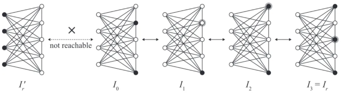
I0

I_r′ I1 I2 I3 = I_r

not reachable

Figure 1.6: A sequence ⟨I0, I1, I2, I3⟩ of independent sets under TAR for the lower

bound l = 1, where the vertices in independent sets are colored with black.

ity variant of independent set reconfiguration. In Opt-ISR, we are given a single solution I0 (an independent set of cardinality at least l), and asked to find

another solution Isol (an independent set) such that it can be reachable from the

ini-tial solution and the cardinality is maximized; we call such a solution Isol an output

solution.

Note that Isol is not always a maximum independent set of an input graph G. For

example, the graph in Figure 1.6 has a unique maximum independent set I_r′ of size four (consisting of the vertices on the left side), but I0 cannot be transformed into

it. Indeed, one of output solutions is I3 for this example when l = 1.

In Chapter 5, we study Opt-ISR from the viewpoints of polynomial-time solv-ability and fixed-parameter (in)tractsolv-ability.

1.3.2 Known and related results

Although Opt-ISR is being introduced in this thesis, some previous results for Reach-ISR are related in the sense that they can be converted into results for Opt-ISR. We present such results here.

Ito et al. [18] showed that Reach-ISR under TAR is PSPACE-complete. On the other hand, Kami´nski et al. [22] proved that any two independent sets of size at least l + 1 are reachable under TAR with the lower bound l for even-hole-free graphs. Reach-ISR has been studied well from the viewpoint of fixed-parameter

(28)

(in)tractability. Mouawad et al. [26] showed that Reach-ISR under TAR is W[1]-hard when parameterized by the lower bound l and the length of a desired sequence (i.e., the number of token additions and removals). Lokshtanov et al. [24] gave a fixed-parameter algorithm to solve Reach-ISR under TAR when parameterized by the lower bound l and the degeneracy d of an input graph.

From our problem setting, one may be reminded of the concept of local search algorithms [1, 30]. To the best of our knowledge, known results for this concept do not have direct relations to our problem, because they are usually evaluated exper-imentally. In addition, note that our problem assumes that an initial independent set I0 is given as an input. In contrast, a local search algorithm is allowed to choose

the initial solution, sometimes randomly.

1.3.3 Our contribution

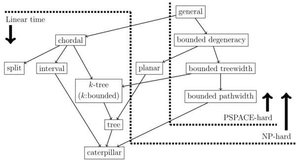
We first study the polynomial-time solvability of Opt-ISR with respect to graph classes, as summarized in Figure 1.7. More specifically, we show that Opt-ISR is PSPACE-hard even for bounded pathwidth graphs, and remains NP-hard even for planar graphs. On the other hand, we give a linear-time algorithm to solve the problem for chordal graphs. We note that our algorithm indeed works in polynomial time for even-hole-free graphs (which form a larger graph class than that of chordal graphs) if the problem of finding a maximum independent set is solvable in polyno-mial time for even-hole-free graphs; currently, its complexity status is unknown.

We next study the fixed-parameter (in)tractability of Opt-ISR, as summarized in Table 1.3. In this paper, we consider mainly the following three parameters: the degeneracy d of an input graph, a lower bound l on the size of independent sets, and the size s of an output solution reachable from a given independent set I0. As

shown in Table 1.3, we completely analyze the fixed-parameter (in)tractability of the problem according to these three parameters; details are explained below.

(29)

general

chordal bounded degeneracy

split interval planar bounded treewidth

k-tree

(k:bounded) bounded pathwidth

tree

caterpillar Linear time

PSPACE-hard NP-hard

Figure 1.7: Our results for Opt-ISR, where each square corresponds to a graph class, and A→ B means that A contains B as a subclass.

We first consider the problem parameterized by a single parameter. We show that the problem is fixed-parameter intractable when only one of d, l, and s is taken as a parameter. In particular, we prove that Opt-ISR is PSPACE-hard for a fixed constant d and remains NP-hard for a fixed constant l, and hence the problem does not admit even an XP algorithm for each single parameter d or l under the assumption that P ̸= PSPACE or P ̸= NP. On the other hand, Opt-ISR is W[1]-hard for s, and admits an XP algorithm with respect to s.

We thus consider the problem taking two parameters. However, the problem still remains NP-hard for a fixed constant d + l, and hence it does not admit even an XP algorithm for d+l under the assumption that P̸= NP. Note that the combination of l and s is meaningless, since we can assume without loss of generality that l + s≤ 2s. On the other hand, we give a fixed-parameter algorithm when parameterized by

s + d; this result implies that Opt-ISR parameterized only by s is fixed-parameter

(30)

Table 1.3: Our results for Opt-ISR with respect to parameters.

(no parameter) lower bound l solution size s (no parameter) NP-h. for fixed l W[1]-h., XP

— (i.e., no FPT, no XP) (i.e., no FPT) [Corollary 5.1] [Theorems 5.4, 5.5] degeneracy d PSPACE-h. for fixed d NP-h. for fixed d + l FPT

(i.e., no FPT, no XP) (i.e., no FPT, no XP)

(31)

18 Chapter 2 Preliminaries

Chapter 2 Preliminaries

2.1 Graph-theoretical terminologies

In this section, we give the basic graph-theoretical terminologies [8, 10].

2.1.1 Graphs and subgraphs

A graph is a ordered pair (V, E), where V is a set of vertices and E ⊆ V × V is a set of edges; we simply denote by uv the edge (u, v). We sometimes denote by V (G) and E(G) the vertex set and the edge set of G, respectively. A graph G is called

simple if G does not contain an edge e = vv for all vertices v ∈ V (G) and more

than two edges e = uv for any pair of two vertices u, v∈ V (G). A graph G is called

undirected if uv ∈ E(G) if and only if vu ∈ E(G); in this case, we identify uv and vu. In this thesis, we consider simple undirected graphs unless otherwise stated.

For an edge e = uv, we say that u and v are adjacent; in this case, u is neighbor

of v, and symmetrically v is neighbor of u. We call each of u and v an endpoint of e, and we say that e is incident to u and v. For a vertex v, the (open) neighborhood

of v in G, denoted by NG(v), is the set of all neighbors of v in G, and the closed

neighborhood of v in G, denoted by NG[v], is defined as NG(v)∪ {v}.

For a graph G = (V, E), a subgraph of G is a graph G′ = (V′, E′) such that both

V′ ⊆ V and E′ ⊆ E hold. In particular, it is a spanning subgraph of G if V′ = V holds. For a graph G = (V, E) and a vertex subset S ⊆ V , a subgraph induced by

S is the subgraph G′ = (V′, E′) where V′ = S and E′ = {uv ∈ E | u, v ∈ S}; we say that S induces G′. On the other hand, for an edge subset U ⊆ E, a subgraph

(32)

2.1 Graph-theoretical terminologies 19

induced by U is the subgraph G′ = (V′, E′) where V′ = ∪_uv_∈U{u, v} and E′ = U ; we say that U induces G′. For a vertex subset S ⊆ V (resp. an edge subset U ⊆ E), we denote by G[S] (resp. G[U ]) the subgraph of G induced by S (resp. induced by

U ).

2.1.2 Path, cycle, and connectivity

Let G = (V, E) be a graph. For two vertices u, v ∈ V , a walk from u to v is a sequence of vertices W = ⟨u = v0, v1, . . . , vℓ = v⟩ such that there is an edge vivi+1 for each i ∈ {0, 1, . . . , ℓ − 1}. ℓ is the length of the walk W. A walk W is called path if all vertices v0, v1, . . . , vℓ inW are distinct. On the other hand, a walk W of length at least three is called cycle if v0 = vℓ and vertices v0, v1, . . . , vℓ−1 are distinct. We sometimes consider a walk (similarly, path and cycle) to be a graph whose vertex set is {v0, v1, . . . , vℓ} and edge set is {vivi+1| i ∈ {0, 1, . . . , ℓ − 1}}.

For a graph G and two vertices u, v ∈ V , the distance between u and v is the minimum ℓ such that there exists a path between u and v of length ℓ; we denote by distG(u, v) the distance between u and v on G. If there is no path between u and v, we consider that the distance between u and v is infinite. G is connected if there is a path between every pair of two vertices in G, and is disconnected otherwise. For a connected graph G, a vertex v ∈ V (G) is called a cut-vertex if G[V (G) \ {v}] is disconnected. For a connected graph G, the diameter of G is the longest distance among all pairs of two vertices in G, that is, maxu,v∈V (G)distG(u, v).

2.1.3 Independent set and clique

For a graph G = (V, E), a vertex subset I ⊆ V is an independent set if no two vertices are adjacent. On the other hand, a vertex subset C ⊆ V is a clique if any two vertices are adjacent.

(33)

2.1.4 Graph classes and parameters

In this subsection, we give the definitions of graph classes and graph parameters which we deal with in this thesis. We first list the definitions of graph classes in the following.

- Tree: A graph is tree if it is connected and contains no cycle as a subgraph. - Cactus: A graph is cactus if every edge is part of at most one cycle.

- Planar: A graph is planar if it can be embedded in the plane without crossing

edges.

- Complete: A graph is complete if any two vertices in the graph are adjacent. - Split: A graph G is split if its vertex set can be partitioned into an independent

set I ⊆ V (G) and a clique C = V (G) \ I.

- Bipartite: A graph G is bipartite if its vertex set can be partitioned into two

independent sets I1 ⊆ V (G) and I2 = V (G)\ I1. In particular, it is complete

bipartite or biclique if any pair of vertices v1 ∈ I1 and v2 ∈ I2 are adjacent.

- Cograph: A graph G is cograph if it contains no path of four vertices as an

induced subgraph.

- Chordal: A graph is chordal if it contains no cycle of more than four vertices as

an induced subgraph.

- Interval: A graph G with V (G) = {v1, v2, . . . , vn} is interval if there exists a set I of (closed) intervals I1, I2, . . . , In such that vivj ∈ E(G) if and only if

Ii∩ Ij =∅ for each i, j ∈ {1, 2, . . . , n}. We call the set I of intervals an interval

representation of G.

We then list the definitions of graph parameters.

- Treewidth: For a graph G, a tree-decomposition of G is a tree T = (B, F ) such

thatB = {B1, B2, . . . , Bk} is the family of vertex subsets of G (each vertex subset inB is called a bag) and T satisfies the following three conditions:

(34)

2.2 Algorithm-theoretical terminologies 21

(a) each vertex v ∈ V (G) belongs to at least one bag, that is ∪_B_∈BB = V (G);

(b) for each edge uv ∈ E(G), there exists at least one bag which contains both

u and v; and

(c) for each vertex v ∈ V (G), all bags containing v forms a subtree of T . The width of a tree-decomposition is defined as maxi|Bi| + 1. The treewidth of G is the minimum t such that G has a tree-decomposition of width t.

- Pathwidth: For a graph G, a tree-decomposition T is also called a

path-decomposition if T is a path. The pathwidth of G is the minimum p such that G

has a path-decomposition of width p.

- Bandwidth: For a graph G, the bandwidth of G is the minimum b such that there

is an injection i : V (G)→ {1, 2, . . . , |V |} such that maxuv∈E(G)|i(u) − i(v)| ≤ b.

- Degeneracy: For an integer d ≥ 0, a graph G is called a d-degenerate graph

if every induced subgraphs of G has a vertex of degree at most d [23]. The

degeneracy of G is the minimum integer d such that G is a d-degenerate graph.

2.2 Algorithm-theoretical terminologies

In this section, we give the basic algorithm-theoretical terminologies [10, 28].

2.2.1 Problems and reductions

An abstract problem is defined to be a binary relation on a set I of problem

instances and a set S of problem solutions. Note that an instance may have more

than one solution. An abstract problem is called a decision problem if each instance has a solution either “yes” or “no” solution, that is, problem solutions S consists of

{0, 1}. Many abstract problems are not decision problems, but rather optimization problems, which require some value to be minimized or maximized. For example,

the reachability variant of a reconfiguration problem is a decision problem, while the optimization variant is not a decision problem but an optimization problem. To

(35)

solve an abstract problem by computers, we must represent the problem as a binary string. Thus we sometimes assume that an abstract problem is represented as a binary string. Then we say that an algorithm solves an abstract problem in time

O(T (n)) if it can output a solution for any instance of length n in time O(T (n)). An

abstract problem is polynomial-time solvable if there exists an algorithm solving the problem in time O(nk_{) for some constant k; such an algorithm is called a}

polynomial-time algorithm.

Let P, P′ be decision problems represented as binary strings. A polynomial-time

reduction from P′ toP is an algorithm which computes an instance I of P for any given instance I′ of P′ such that;

- the solution of I in P is “yes” if and only if that of I′ inP′ is “yes;” and

- the algorithm runs in time O(nk_{), where n =} _|I′_{| is the length of the instance I} and k is some constant.

An abstract problem parameterized by p is defined to be a binary relation on a set Ip of problem instances and a set S of problem solutions, where Ip is a set of pairs consist of an instance of an abstract problem and a natural number, called

parameter; we call an abstract problem parameterized by some parameter a param-eterized problem. Then an abstract problem paramparam-eterized by p is fixed-parameter tractable if there exists an algorithm which can be output a solution for any instance

(I, p) in time O(f (p)· nk_{), where f is some computable function depending only on}

p, n = |(I, p)| is the length of the instance (I, p), and k is some constant; we call

such an algorithm a fixed-parameter algorithm or an FPT algorithm. On the other hand, we call an algorithm an XP algorithm if it runs in time O(nf (k)_{) where f is} an arbitrary function depending only on k.

LetP and P′ be decision problems parameterized by p and p′, respectively. Then, a parameterized reduction (or an FPT reduction) is an algorithm which computes an instance (I, p) of P for any given instance (I′, p′) of P′ such that;

(36)

2.2 Algorithm-theoretical terminologies 23

- the solution of (I, p) in P is “yes” if and only if that of (I′, p′) in P′ is “yes;”

- p ≤ g(p′) holds for some computable function g depending only on p′; and

- the algorithm runs in time O(f (p′)· nk_{), where f is some computable function} depending only on p′, n =|(I′, p′)| is the length of the instance (I′, p′), and k is some constant.

2.2.2 Class of computational complexity

In this subsection, we describe some classes of problems with respect to compu-tational complexity.

NP is the class of all decision problems that can be verified by a polynomial-time

algorithm. An abstract problem P is NP-hard if for any problem P′ in NP, there is a polynomial-time reduction from P′ toP. A decision problem P is NP-complete if it is NP-hard and in NP. Note that there is no polynomial-time algorithm solving an NP-hard problem, unless P = NP.

PSPACE is the class of all abstract problems that can be solved in polynomial

space. An abstract problem P is PSPACE-hard if for any problem P′ in PSPACE, there is a polynomial-time reduction from P′ to P. An abstract problem P is

PSPACE-complete if it is PSPACE-hard and in PSPACE. Note that there is no

polynomial-time algorithm solving a PSPACE-hard problem, unless P = PSPACE.

XP and FPT is the class of all parameterized problems that can be solved by an XP

algorithm and an FPT algorithm, respectively. Note that FPT is a subclass of XP.

W[1] is the class of all parameterized problems such that for any problemP in W[1],

there is a parameterized reduction from it to weighted 2-cnf-satisfiability. A parameterized problem P is W[1]-hard if for any problem P′ in W[1], there is a parameterized reduction fromP′ toP. Note that there is no FPT algorithm solving a W[1]-hard problem, unless FPT = W[1].

(37)

24 Chapter 3 Reconfiguration of fundamental graphs

Chapter 3 Reconfiguration of

fundamental graphs

In this chapter, we study the complexity of the reachability variant of reconfiguration problems with several graph properties.

3.1 Definition of problems and preliminaries

We formally define the reconfiguration problems of subgraphs satisfying a funda-mental property; the property subgraphs must satisfy is specified as property Π. Let

G be an input graph. Feasible solutions are defined as subgraphs satisfying Π. More

specifically, we consider three versions according to how to represent subgraphs; in each version, a feasible solution is defined, as follows:

- Edge version: an edge subset U ⊆ E(G) such that G[U] satisfies Π.

- Induced version: a vertex subset S ⊆ V (G) such that G[S] satisfies Π.

- Spanning version: a vertex subset S ⊆ V (G) such that G[S] contains at least

one spanning subgraph satisfying Π.

Then, we consider the following two adjacency relations:

- Token-jumping (TJ, for short): Tow feasible solutions S, S′(edge subsets in the edge version, and vertex subsets in the induced and spanning version) are adjacent

under TJ if |S \ S′| = |S′\ S| = 1 holds.

- Token-sliding (TJ, for short): In the edge version, two feasible solutions U, U′ ⊆

E(G) are adjacent under TS if |U \ U′| = |U′\ U| = 1 holds and the unique edges e ∈ U \ U′ and e′ ∈ U′\ U have a common end point in G. In the induced and

(38)

3.2 General XP algorithm 25

spanning versions, two feasible solutions S, S′ ⊆ V (G) are adjacent under TJ if

|S \ S′_{| = |S}′_{\ S| = 1 holds and the unique vertices v ∈ S \ S}′ _{and v}′ _{∈ S}′ _{\ S} are adjacent in G.

Then, we deal with the reachability variant of reconfiguration problems whose solu-tion spaces are defined above. More specifically, for a property Π and an adjacency relation R ∈ {TJ, TS}, we consider the following problem: We are given a graph

G and two feasible solutions S0 and Sr in the solution space, then asked to

deter-mine whether or not there exists a reconfiguration sequence between S and S′ in the solution space.

We denote by (G, V0, Vr) an instance of a spanning version or an induced version whose input graph is G and source and target solutions are vertex subsets V0 and

Vr of G. Similarly, we denote by (G, E0, Er) an instance of the edge version. We may assume without loss of generality that |V0| = |Vr| holds for the spanning and induced versions, and |E0| = |Er| holds for the edge versions; otherwise, the answer is clearly no since under both the TJ and TS rules, all solutions must be of the same size.

3.2 General XP algorithm

In this section, we give a general XP algorithm when the size of a solution (that is, the size of a vertex or edge subset that represents a subgraph) is taken as the parameter. For notational convenience, we simply use element to represent a vertex (or an edge) for the spanning and induced versions (resp., the edge version), and

candidate to represent a set of elements (which does not necessarily satisfy the

property Π). Furthermore, we define the size of a given graph as the number of elements in the graph.

Theorem 3.1 Let Π be any graph structure property such that we can check if a

(39)

depending only on k. Then, all of the spanning, induced, and edge versions under

TJ or TS can be solved in time O(n2kk + nkf (k)), where n is the size of a given graph and k is the size of a source (and target) solution. Furthermore, a shortest reconfiguration sequence between source and target solutions can be found in the same time bound, if it exists.

Proof. Our claim is that the reconfiguration graph can be constructed in the stated

time. Since a given source solution is of size k, it suﬃces to deal only with candidates of size exactly k. For a given graph, the total number of possible candidates of size

k is O(nk). For each candidate, we can check in time f (k) whether it satisfies Π. Therefore, we can construct the node set of the reconfiguration graph in time

O(nk_{f (k)). We then obtain the edge set of the reconfiguration graph. Since there} are O(nk) nodes in the reconfiguration graph, the number of pairs of nodes is O(n2k). Since each node corresponds to a set of k elements, we can check if two nodes are adjacent or not in O(k) time. Therefore, we can find all pairs of adjacent nodes in time O(n2k_k).

In this way, we can construct the reconfiguration graph in time O(n2k_k+nk_{f (k)) in} total. The reconfiguration graph consists of O(nk) nodes and O(n2k) edges. There-fore, by breadth-first search starting from the node representing a given source solu-tion, we can determine in time O(n2k_{) whether or not there exists a reconfiguration}

sequence between two nodes representing the source and target solutions. Notice that if a desired reconfiguration sequence exists, then breadth-first search finds a

shortest one. 2

3.3 Edge versions

In this section, we study the edge version for five diﬀerent properties, namely those specifying that the graph be a path, a cycle, a clique, a biclique, or a tree.

(40)

3.3 Edge versions 27 s t v x s 1 s2 sn sn+1 t 1 t2 tn tn+1 w e 1 en e 1 en e_n+1 e n+1 e 1 e2 e3 G P s P t s s s t t _t

Figure 3.1: Reduction to the edge version under TJ for the property “a graph is a path.”

We first consider the property “a graph is a path” under TJ.

Theorem 3.2 The edge version under TJ is NP-hard for the property “a graph is

a path.”

Proof. We give a polynomial-time reduction from the Hamiltonian path problem.

Recall that a Hamiltonian path in a graph G is a path that visits each vertex of G exactly once. Given a graph G and two vertices s, t∈ V (G) of G, the NP-complete problem Hamiltonian path is to determine whether or not G has a Hamiltonian path which starts from s and ends in t [14].

For an instance (G, s, t) of Hamiltonian path, we construct a corresponding in-stance (G′, Es, Et) of our problem, as follows. (See also Figure 3.1.) Let n =|V (G)|. We first add two new vertices v and x to G with two new edges e1 = xv and e2 = vs.

We then add two paths Ps =⟨s1, s2, . . . , sn+1, x⟩ and Pt=⟨t1, t2, . . . , tn+1, x⟩, where

s1, s2, . . . , sn+1 and t1, t2, . . . , tn+1 are distinct new vertices. Each of Ps and Pt con-sists of n+1 edges; we denote by es

1, es2, . . . , esn+1the edges s1s2, s2s3, . . . , sn+1x in Ps, respectively, and by et₁, et₂, . . . , et_n+1the edges t1t2, t2t3, . . . , tn+1x in Pt, respectively. We finally add a new vertex w with an edge e3 = tw, completing the construction

of G′. We then set Es = {es1, es2, . . . , esn+1, e1, e2} and Et = {et1, e2t, . . . , etn+1, e1, e2};

these edge subsets clearly form paths in G′. We have thus constructed our corre-sponding instance (G′, Es, Et) in polynomial time.

(41)

if and only if the corresponding instance (G′, Es, Et) is a yes-instance.

To prove the only-if direction, we first suppose that G has a Hamiltonian path

P starting from s and ending in t. Then, we construct an actual reconfiguration

sequence from Es to Et using the edges in P . Notice that P consists of n− 1 edges. Thus, we first move the n− 1 edges es

1, es2, . . . , esn−1 in Es to the edges in P one by one, and then move es

n to e3. Next, we move esn+1 to etn+1, and then move the edges in E(P )∪ {e3} to etn, etn−1, . . . , et1 one by one. By the construction of G′, we know

that each of the intermediate edge subsets forms a path in G′, as required.

We now prove the if direction by supposing that there exists a reconfiguration sequence⟨Es = E0, E1, . . . , Eℓ = Et⟩. Let Eq be the first edge subset in the sequence such that E(Pt)∩Eq ̸= ∅; we claim that Eqcontains a Hamiltonian path in G. First, notice that the edge in E(Pt)∩ Eq is etn+1; otherwise the subgraph formed by Eq is disconnected. Since|Eq| = |Es| = n+3 and |E(Ps)| = n+1, we can observe that Eq contains no edge in Ps; otherwise the degree of x would be three, or Eq would form a disconnected subgraph. Therefore, the n + 2 edges in Eq\ {etn+1} must be chosen from E(G)∪ {e1, e2, e3}. Since |V (G)| = n and Eq must form a path in G′, we know that Eq\{etn+1} consists of e1, e2, e3and n−1 edges in G. Thus, Eq\{etn+1, e1, e2, e3}

forms a Hamiltonian path in G starting from s and ending in t, as required. 2 We now consider the property “a graph is a cycle,” as follows.

Theorem 3.3 The edge version under each of TJ and TS can be solved in linear

time for the property “a graph is a cycle.”

Proof. Let (G, Es, Et) be a given instance. We claim that the reconfiguration graph is edgeless, in other words, no feasible solution can be transformed at all. Then, the answer is yes if and only if Es = Et holds; this condition can be checked in linear time.

Let E′be any feasible solution of G, and consider a replacement of an edge e−∈ E′ with an edge e+ _{other than e}−_{. Let u, v be the endpoints of e}−_{. When we remove}

(42)

3.3 Edge versions 29

e− from E′, the resulting edge subset E′ \ {e} forms a path whose ends are u and

v. Then, to ensure that the candidate forms a cycle, we can choose only e−= uv as

e+_{. This contradicts the assumption that e}+ _{̸= e}−_. ₂

The same arguments partially hold for the property “a graph is a clique,” and we obtain the following theorem. We note that, for this property, both induced and spanning versions (i.e., when solutions are represented by vertex subsets) are PSPACE-complete under any adjacency relation [19].

Theorem 3.4 The edge version under each of TJ and TS can be solved in linear

time for the property “a graph is a clique.”

Proof. Suppose that (G, Es, Et) be a given instance. If the size of the clique (the number of vertices of the subgraph) formed by Es (and Et) is at least three, then the same arguments in the proof of Theorem 3.3 hold, and hence the instance can be solved in linear time. We thus consider the other case where Es and Et form 2-cliques. In this case, we know |Es| = |Et| = 1. Then, under TJ, we observe that it is always a yes-instance, since we can move the unique edge in Es into that in Et directly. On the other hand, under TS, we observe that it is a yes-instance if and only if Es and Et are contained in the same connected component of G. Therefore, we can conclude that this case is also solvable in linear time. 2

We next consider the property “a graph is an (i, j)-biclique,” as follows.

Theorem 3.5 The edge version under each of TJ and TS can be solved in

poly-nomial time for the property “a graph is an (i, j)-biclique” for any pair of positive integers i and j.

Proof. We may assume without loss of generality that i ≤ j holds. We prove the theorem in the following three cases:

- Case 1: i = 1 and j ≤ 2; - Case 2: i, j ≥ 2; and

(43)

- Case 3: i = 1 and j ≥ 3.

We first consider Case 1, which is the easiest case. In this case, any (1, j)-biclique has at most two edges. Therefore, by Theorem 3.1 we can conclude that this case is solvable in polynomial time.

We then consider Case 2. We show that (G, Es, Et) is a yes-instance if and only if Es = Et holds. To do so, we claim that the reconfiguration graph is edgeless, in other words, no feasible solution can be transformed at all. To see this, because

i, j ≥ 2, notice that the removal of any edge e in an (i, j)-biclique results in a

bipartite graph with the same bipartition of i vertices and j vertices. Therefore, to obtain an (i, j)-biclique by adding a single edge, we must add back the same edge e. We finally deal with Case 3. Notice that a (1, j)-biclique is a star with j leaves, and its center vertex is of degree j ≥ 3. Then, we claim that (G, Es, Et) is a yes-instance if and only if the center vertices of stars represented by Es and Et are the same. The if direction clearly holds, because we can always move edges in Es\ Et into ones in Et\Esone by one. We thus prove the only-if direction; indeed, we prove the contrapositive, that is, the answer is no if the center vertices of stars represented by Es and Et are diﬀerent. Consider such a star Ts formed by Es. Since Ts has

j (≥ 3) leaves, the removal of any edge in Es results in a star having j − 1 (≥ 2) leaves. Therefore, to ensure that each intermediate solution is a star with j leaves, we can add only an edge of G which is incident to the center of Ts. Thus, we cannot

change the center vertex. 2

In this way, we have proved Theorem 3.5. Although Case 1 takes non-linear time, our algorithm can be easily improved under TJ so that it runs in linear time; in Case 1, a subgraph forms a (1, j)-biclique if and only if it forms a tree, and hence we can solve in linear time by Theorem 3.6 (presented later).

We finally consider the property “a graph is a tree” under TJ. As we have men-tioned in the introduction, for this property, there are several choices of trees even

東北大学機関リポジトリTOUR

Reconfiguration of Subgraphs Satisfying

Specific Properties

著者

水田 遥河

学位授与機関

Tohoku University

学位授与番号

11301甲第19346号

URL

http://hdl.handle.net/10097/00130236

Reconfiguration of Subgraphs Satisfying

Specific Properties

by

Haruka Mizuta

Submitted to

Department of System Information Sciences

in partial fulfillment of the requirements for the degree of

Doctor of Philosophy (Information Sciences)

Graduate School of Information Sciences

Tohoku University, Japan

Acknowledgements

Abstract

Contents

List of Figures

Chapter 1

Introduction

1.1

Combinatorial reconfiguration

1.2

Reconfiguration of (connected) subgraphs

1.2.1

Our problems

ʹ

ʹ

ʹ

1.2.2

Known and related results

1.2.3

Our contribution

1.3

New variant of reconfiguration problems

1.3.1

Our problem

1.3.2

Known and related results

1.3.3

Our contribution

Chapter 2

Preliminaries

2.1

Graph-theoretical terminologies

2.1.1

Graphs and subgraphs

2.1.2

Path, cycle, and connectivity

2.1.3

Independent set and clique

2.1.4

Graph classes and parameters

2.2

Algorithm-theoretical terminologies

2.2.1

Problems and reductions

2.2.2

Class of computational complexity

Chapter 3

Reconfiguration of

fundamental graphs

3.1

Definition of problems and preliminaries

3.2

General XP algorithm

3.3

Edge versions

水田遥河