JAIST Repository: A Study on Long-Short Term Memory Networks with Attention Mechanism

(1)

JAIST Repository

https://dspace.jaist.ac.jp/

Title A Study on Long-Short Term Memory Networks with Attention Mechanism

Author(s) Su, Hang

Citation

Issue Date 2019-03

Type Thesis or Dissertation

Text version author

URL http://hdl.handle.net/10119/15817

Rights

Description Supervisor: Huynh Nam Van, 先端科学技術研究科, 修

(2)

A Study on Long-Short Term Memory Networks with

Attention Mechanism

SU HANG

School of Knowledge Science,

Japan Advanced Institute of Science and Technology

March 2019

Keywords: Natural language processing, sentiment analysis, text data, machine learning,

deep learning, Long short term memory, LSTM, Bi-LSTM, attention mechanism

With the rapid development of e-commerce websites, more and more people choose online shopping, which generates a large number of product review information. Sentiment analysis of text information not only tap customers' preference for products and provide shopping suggestions to potential customers, but also can help providers to improve products and services in a timely manner and improve business value.

Therefore, it is very necessary to classify product reviews by sentiment. There are two traditional research methods of sentiment classification: (1) the method based on lexicon; (2) methods based on machine learning. The former requires creating the lexicon manually, which is laborious. The latter is usually classified by naive bayes (NB), maximum entropy (ME), support vector machine (SVM), etc. These methods are easy to lose the syntactic and semantic information of the text and difficult to effectively capture the sentiment in the text.

With the application of deep neural networks in the field of natural language processing, Bengio et al. used neural networks to train word vectors to represent texts in 2003. The word vector can not only obtain semantic information effectively, but also avoid the problem of data sparsity. The word vector is used to represent the text, and by using the deep learning model, such as multi-layer neural network, convolutional neural network (CNN), recurrent neural network (RNN), etc., is adopted for sentiment classification, which can achieve better

(3)

results than traditional machine learning methods.

Considering that the text data has strongly dependent on the context when classifying product reviews, and the standard neural network model cannot well solve the problem, so in this study, I adopted the Bidirectional Long Short term Memory neural network (Bi-LSTM) for sentiment analysis. In addition, considering the different contributions of different words to the text, the Attention mechanism is introduced. Based on this, this study proposes a Bi-LSTM model based on the Attention mechanism to classify product reviews.

In order to verify the validity of the model, this study used the dataset of SemEval(International Workshop on Semantic Evaluation) 2014 Task 4 which is composed of reviews in Restaurant and Laptop. to test the model. Finally the experimental results show that the model is effective.

(4)

List of Figures

Figure 1 the schematic diagram of SVM ... 16

Figure 2 schematic diagram of classification hyperplane ... 17

Figure 3 An example of gradient descent ... 25

Figure 4 Sigmoid function graph ... 26

Figure 5 the structure of CBOW... 30

Figure 6 the structure of Skip-gram ... 31

Figure 7 shown the semantic relationship through the vector space ... 33

Figure 8 the network topology of single neural unit ... 34

Figure 9 network structure of MLPs... 36

Figure 10 An example of the application of convolutional neural networks in the image classification ... 37

Figure 11 the structure of sentiment analysis ... 38

Figure 12 the structure of RNN ... 40

Figure 13 the tanh layer in RNN unit ... 41

Figure 14 the structure of LSTM ... 42

Figure 15 the key of LSTM ... 42

Figure 16 activation operation ... 43

Figure 17 forget gate ... 44

Figure 18 input gate ... 44

Figure 19 updating the state of cell 𝐶𝑡 ... 45

Figure 20 output gate ... 45

Figure 21 the structure of Bi-LSTM ... 46

Figure 22 Global Attention Model and Local Attention Model ... 48

Figure 23 shown the structure of attention layer ... 49

Figure 24 the sample of datasets ... 51

(7)

Figure 26 Confusion Matrix ... 56

Figure 27.1 MLP2560 with random Figure 27.2 MLP2560 with word2vec ... 57

Figure 27.3 Train accuracy and loss of LSTM256 Figure 27.4 CNN1200 ... 57

(8)

List of charts

Chart 1 Structures of all experiments ... 53

Chart 2 Structures of each MLPs ... 53

Chart 3 Structures of each CNN ... 53

Chart 4 Structures of each LSTM ... 54

Chart 5 Structures of each Bi-LSTM ... 54

Chart 6 the results of all models with random representation ... 59

(9)

List of formula

Formula 1 The input and output expressions of the perceptron ... 21

Formula 2 expressions of the perceptron ... 21

Formula 3 ... 22 Formula 4 ... 22 Formula 5 ... 23 Formula 6 ... 23 Formula 7 ... 23 Formula 8 ... 23 Formula 9 ... 24 Formula 10 ... 24 Formula 11 ... 24 Formula 12 ... 25 Formula 13 ... 26

Formula 14 the sigmoid function ... 26

Formula 15 the derivative of sigmoid function ... 27

Formula 16 the derivative of tanh function ... 27

Formula 17 ... 27

Formula 18 ... 27

Formula 19 ... 28

Formula 20 ... 28

Formula 21 objective function of CBOW ... 29

Formula 22 objective function of Skip-gram ... 31

Formula 23 target word probability of word2vec ... 33

Formula 24 ... 35

Formula 25 ... 40

(10)

Formula 27 ... 50 Formula 28 ... 50 Formula 29 ... 57

(11)

Chapter 1

Introduction

1.1 Background

Existing researches shown as in the earlier study, researchers adopted traditional machine learning methods to solve many tasks of natural language processing(NLP), such as classifying news texts with support vector machines(SVM) [1] or processing spam with naive Bayes[2] etc. But with the rise of social media on the Internet, volume of text data surges, no matter from the workload or from the final test results, the traditional classification methods Fare unable to give satisfactory results, and the emergence of deep learning breaks the deadlock in a certain sense, makes a lot of tasks in the field of natural language processing got breakthrough bottlenecks.

Deep learning has become a powerful machine learning technology that can learn multiple representations or features of data and produce state-of-the-art predictive results. With the success of deep learning in many application fields, deep learning has also been used in emotional analysis in recent years. The representation capability of the deep neural network is not the same as that of the superficial log-linear model (including low-order CRF); many of the architectures that currently achieve the current optimal level of performance on standard datasets basically are variations of multi-tier, bidirectional Recurrent Neural Network (RNN). Many tasks, such as language modeling and machine translation, already have large-scale marked training data or parallel sentence pairs, and the level of training data available for various tasks in the industry is beyond imagination. All of these can only be better fitted with structures which have stronger representation ability. In addition, even for small scale tasks with unlabeled data, we also can use the word vectors trained from massive corpus obtain information, and that can get better describe semantic proximity than BoW discrete vectors obtained from

(12)

classical brown clustering. Even if some words or representations are not seen in the supervised training corpus, but the representation which learned in the unlabeled corpus is close to another common word, the classical approach to semi-supervised learning using massive unlabeled corpus is not so easy.

After the application of deep learning in the field of natural language processing, there are many methods for the sentiment analysis tasks. The earliest research is to use the MLPs to implement the sentiment classification, this method uses the vectors of words in a sentence to calculate the average, this method loses the semantic relations in the sentence, and other researchers tried to use Convolutional neural network (CNN) model, this method is treating a sentence as a feature map, and to calculate the feature maps, Though method has shown its effectives, but for now, for the NPL tasks the most common solution is RNN. The neural network of RNN structure can better preserve the semantic connections in sentences and has better effect on the sequential data such as speech and text data. As a variant of RNN, Long-Short term memory (LSTM) has a better effect on sequential data such as text, while the recently published attention mechanism with neural network, focuses on the dependence of current words in current input.

1.2 Research purposes

To use the supervised learning models, datasets of review sentences annotated with ground-truth sentiment have to be supplied as the training data. The data annotation process involves intense human labor even linguistic expertise, therefore, the availability of the training data is usually very limited.

In addition to the problem above, the review data is full of comparative and shifting opinions; therefore, the boundaries separating different opinion classes should be highly non-linear. And traditional learning models, such as SVM, Naïve Bayes, Logistic regression, etc., are not strong enough to capture the non-linearity.

(13)

This study will consider the combination of attention mechanism and LSTM model to achieve better classification effect in sentiment analysis task.

(14)

Chapter 2

Related Work

2.1 Sentiment analysis

Sentiment analysis (SA) [3], also known as tendency analysis and opinion mining, is a process of analyzing, processing, summarizing and reasoning for subjective texts with emotion. Among them, sentiment analysis can be further divided into sentiment polarity (tendency) analysis, sentiment degree analysis, subjective and objective analysis, etc. The purpose of polarity analysis of sentiments to judge the positive, negative and neutral meanings of the text. In most application scenarios, there are only two categories. For example, the words "like" and "dislike" belong to different sentiment tendencies. Sentiment degree analysis is mainly to divide or subdivide the same sentiment polarity to describe the intensity of the polarity. For example, "like" and "love" are both positive terms, but "love" is relatively more positive. Subjective and objective analysis is to distinguish which parts of the text are objective statements without emotional color and which are emotional description.

2.1.1 Major methods of sentiment analysis

At present, there are two main types of sentiment analysis methods: lexicon-based method and machine learning-based method.

The lexicon-based method mainly makes use of a series of affective dictionaries and rules, breaks the text into paragraphs, analyzes the syntax, and calculates the affective value. Finally, the affective value is taken as the basis of the emotional tendency of the text. There a lot of sentiment lexicons, such as General Inquirer [4]; LIWC [5]; MPQA Subjectivity Cues Lexicon [6]; Bing Liu Opinion Lexicons [7]; SentiWordNet [8].

(15)

problem. For the judgment of sentiment polarity, target sentiments are classified into two categories: positive and negative. The training text is marked manually and then the supervised machine learning process is carried out. For example, machine learning based on large-scale corpus is quite common, Such as GLOVE, word2vec, etc.

2.1.1.(i) Lexicon-based method

Sentiment minimum granularity analysis object is word, but the most basic unit to express sentiment is sentence, words can describe the basic information of the emotion, but a single word without object, context, maybe at different emotion environment, the same word combinations have opposite emotional tendencies. Therefore, it is reasonable to use sentences as the most basic granularity of sentiment analysis. The sentiment of a passage or paragraph can be calculated by the sentiment of sentence.

The general steps of lexicon-based sentiment analysis are as follows: 1. Divide into paragraphs;

2. Divide sentences in each paragraph; 3. Divide words in each sentence;

4. Search for sentiment words and label and count them;

5. Search the degree words before sentiment words, according to the degree, give different weights;

6. Search for negative words before sentiment words, and assign inversion weight; 7. Calculate the sentiment score of the sentence;

8. Calculate the sentiment score of the paragraph; 9. Calculate the sentiment score of the article;

Considering that the sentence is not a stable distribution, the above steps process positive and negative emotion words respectively, and the final two score represent the positive sentiment score and negative sentiment score of the text respectively.

(16)

Algorithm design (pseudo code):

1:fetch all text 2:for each text:

3: for each parameter in text: 4: for each sentence in parameter: 5: for each word in sentences:

6: if word in sentiment_dicts:

7: if adverb before sentenceword

8: score = adverb*score

9: if inverse before sentenceword

10: score = -1 * score

After the steps above, each sentence of each paragraph from each article will have a corresponding sentiment score. Then, according to the needs, the score of the sentence can be statistically calculated, and the score of the paragraph also can be statistically calculated, so as to obtain the positive sentiment value and negative sentiment value of the final text.

2.1.1.2(ii) Machine learning-based method

(a)Text structuring

Text structuring is an important step in machine learning. Because of the particularity of text, computers cannot directly understand the semantics in text. So we need to structure the text as input to the classifier.

(1)Minimum semantic granularity

In English, the minimum semantic granularity is letters, but a single letter represents too little semantic information. Generally, most words are used as the most basic morpheme, because this is also the case in actual communication. However, as the minimum semantic granularity, there is also a problem that the relationship between words is lost along with the word segmentation.

(17)

In fact, this part of information is very important. In order to reduce this implicit semantic loss, n-gram model has been proposed. The n-gram model is based on the assumption that the appearance of the n word is only related to the previous n-1 word and not to any other word. Simply the min-morpheme corresponding to the unigram model is a single word, and the bigram model is a two-word string. For example, in bigram model "I love Japan very much" is “I love”, ”love Japan”, ”Japan very”, “very much”. Due to the fatal defect of n-gram -- the results are too sparse. Assume that there are 1000 words in the word list of normal word segmentation. If it is bigram, there are 1000000 possible n-grams; if it is trigram, there are 1000000000 possible n-grams, and the dimension growth is exponential.

In general, only two or three strings are used as the minimum semantic granularity in use, and other processing is needed to reduce the dimension and reduce the consumption of computing resources.

(2)Text vectorization

Text vectorization is the most important step in text structuring. If determining the minimum semantic granularity is to tell the computer the minimum unit of semantic information, then vectorization is to tell the computer what structure to use to understand the text. The mainstream representation methods are: bag-of-words (BoW) and vector space model. In fact, these two models are relatively similar. Both of them take the vocabulary (or the smallest morpheme in n-gram) as the minimum particle size of the segmentation, and split a sentence to obtain "I", "love", "Tokyo" and "city". The weight of the word is set according to the number of occurrence of each word, and the word is converted into a vector in the form of [1, 1, 1, 1]. On the basis of the BoW model, the vector space model integrates multiple text word bag models together to form a two-dimension matrix of word-document. Words are also called dimensions or features. In general, lexicon-based affective analysis is based on the former, while the latter is applied to large-scale corpus. The entry weight is in the word bag or word frequency

(18)

matrix. If the word appears, it will be marked as 1; if it does not appear, it will be marked as 0, which is called Boolean weight. People found that some words appeared many times in the article, they should have a more important position, so the Boolean weight was upgraded to the word frequency weight, and the frequency of the word appeared in the article was used as the weight.

Later, it was found that some words had high word frequency in all articles, such as "the". These words have no value to the article, and need to be eliminated to save performance costs. Therefore, people eliminate these words with average distribution by inverse document frequency idf, and the product of word frequency and inverse document frequency is the commonly used tf-idf weight.

(3)Feature extraction

Feature extraction is the last step of text vectorization, and its importance is more reflected in the prevention of model overfitting and the reduction of computing costs without loss of precision. In the face of massive amounts of data, it is no less important than any previous step. There are two main methods of feature extraction: feature selection and feature extraction.

Feature selection is to select the feature dimension that contributes more to the target category in a pile of features, calculate the weight of features, and select a higher part of feature dimension as the input feature of model training according to the weight reordering. The weight here is different from the word (feature) weight that we talked about earlier. Feature weight describes the relationship between features and target categories, while word weight describes the importance of words in articles, which are very easy to be confused.

Feature extraction takes all features as input and outputs a batch of new features through some way or algorithm. The number of dimensions of this feature is much smaller than the length of the original feature. The loss of information in this process is much less than the feature selection. Deep learning and neural networks are the main algorithms.

(19)

(b)Selection of classification algorithm

After the text is structured, it can be trained. Of course, you still need to choose a suitable classifier. In the major literature, the most recommended text classification algorithm is neural network. Because of its excellent generalization ability, neural networks are now favored by the industry and used in many classification occasions. Of course, there are many classifiers, naive bayes, neural network, K approach, Support Vector Machine (SVM) have their own advantages. When the neural network was not concerned, the effect of SVM was very excellent.

SVM is a supervised learning algorithm. The criterion for classification is the maximum classification boundary, and the vector (feature) on the classification boundary is the support vector.

Figure 1 the schematic diagram of SVM

So the vector that is directly involved in the sorting operation is actually smaller than the original input vector. This is also the reason why the performance is better in the

(20)

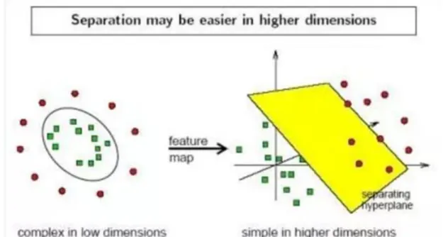
unique to SVM is the classification hyperplane.

Because the data is very complicated in reality, especially text data, the data after vectorization is not a simple linear relation, so there are some people think to solve the problem which is high-dimensional linear inseparable, the figure as shown below is an example, complex relationships in low dimensional space can be mapped to simple linear relationships in high dimensions, Of course, the data in the real world is not that simple, so the mapping from low dimension to high dimension is much more complicated than you think. But there are still some people who have shown mathematically that the problem of low dimensional separately can be linearly separable in higher dimensions, at least in one of the higher dimensions.

Figure 2 schematic diagram of classification hyperplane

2.2 Background knowledge in deep learning

2.2.1 History of Deep learning

In 1958, psychologist Rosenblatt put forward the earliest feed-forward hierarchical network mode [9], which was known as Perceptron. In this model, the input graph is

(21)

allocated to each node of the next layer through each node. This layer is called the middle layer. The middle layer can be one layer or multiple layers, and finally the output graph is obtained through the node of the output layer. In this kind of feed-forward network, there is no feedback connection, no intra-layer connection and no feedforward connection between two layers. Each node can only be feedforward connected to all nodes in the next layer. However, at that time, there was no feasible training method for the multi-layer perceptron with hidden layer, so the perceptron in the initial study was a one-layer perceptron.

In 1969, Minskey and Papert conducted a detailed analysis of the simple perceptron proposed by Rosenblatt. A typical chestnut they cite is the so-called XOR(exclusive -- or) problem. Minskey and Papert point out that simple perceptron without hidden layer is powerless in many cases like XOR problem, and prove that simple perceptron can only solve linear classification problem and first-order predication problem. For nonlinear classification problems and higher-order predicate problems, the hidden element layer must be used. The hidden unit can re-encode the input pattern with a certain weight, Thus, the similar performance of this pattern supports any required input/output mapping in the new encoding, rather than making the mapping difficult to implement as with a simple perceptron.

The general Delta rule proposed by Rumelhart, Hinton and Williams, namely the back propagation algorithm [10], solves this problem well. The learning process of the back propagation algorithm is an error correction learning algorithm, which is composed of forward propagation and back propagation. In the process of forward propagation, the input signal propagates from the input layer to the hidden layer and the output layer, layer by layer after passing through the action function, and the neuron state of each layer only affects the neuron state of the next layer. If the desired output is not obtained at the output layer, it goes into reverse propagation, returning the connection signal along the original connection path. By modifying the connection weight of neurons in each layer, makes the minimum output error signal and back propagation neural network connection structure

(22)

and mapping process is the same as multi-layer Perceptron, only the latter cell activation function was in as a Sigmoid function. Rumelhart et al. rediscovered in 1985 that the sample learning algorithm based on the generalized delta rule [11] could be effectively applied in multi-layer network, which solved the problem of XOR and other learning problems that could not be solved in Perceptron model in the past.

2.2.2 Current status of deep learning

In recent years, the development of deep learning is gradually mature. In June 2012, the New York TIMES revealed the Google Brain project, which attracted wide public attention. The project was led by Andrew Ng, a well-known machine learning professor at Stanford University, and Jeff Dean, the world's leading expert on large-scale computer systems. He trained 16,000 CPU Core parallel computing platforms to train deep neural networks with 1 billion nodes. (Deep Neural Networks, DNN), which enables self-training to identify 14 million images of 20,000 different objects. There is no need to manually enter any features such as "face, body, what a cat looks like" into the system before starting to analyze the data. The system actually invented or understood the concept of 'cat'.

In March 2014, it was also based on the deep learning method. Facebook's DeepFace project made the recognition rate of face recognition technology reach 97.25%, which is only slightly lower than the correct rate of 97.5% of human recognition. The accuracy is almost comparable. Humanity. The project utilizes a 9-layer neural network to obtain facial characterization, with neural network processing parameters of up to 120 million. And in March 2016, the artificial intelligence go game was won by AlphaGo developed by David Silver, Aijia Huang and Daimis Hazabis of DeepMind, a Google-based company in London, England. Li Shishi, the world's Go champion and professional nine-segment player, won with a total score of 4:1. AlphaGo's main working principle is deep learning, which improves the game of chess through two different neural network

(23)

"brains": the first brain: the Move Picker and the second brain: the Position Evaluator. These brains are multi-layered neural networks that are structurally similar to those recognized by Google's image search engine. They start with a multi-layered heuristic 2D filter to handle the positioning of the Go board, just like the image classifier network processes the image. After filtering, the 13 fully connected neural network layers produce a judgment of what they see. These layers are capable of doing classification and logical reasoning.

(24)

Chapter 3

Approach

3.1 Deep learning algorithm

In order to solve the above shortcomings, the deep learning-based algorithm is adopted for sentiment analysis in this study. In the deep learning model, almost all neuron units are implemented by perceptron algorithm. to understand the processing of deep learning model, I should understand perceptron algorithm first.

3.1.1 Perceptron algorithm

First, 𝑛 as inputs, and each input value are weighted. Then, it is determined whether the input by weighted sum of perceptron reaches a certain threshold value 𝑣 or not. If it does, it outputs 1 through the sign function; otherwise, it outputs -1.

Formula 1 The input and output expressions of the perceptron

To unify the expression, we set the upper threshold 𝑣 to 𝑤₀ and add the variable x₀ = 1 so that we can use 𝑤₀𝑥₀+ 𝑤₁𝑥₁+ 𝑤₂𝑥₂+ ⋯ + 𝑤_𝑛𝑥_𝑛 > 0 instead of 𝑤₀𝑥₀+ 𝑤₁𝑥₁+ 𝑤₂𝑥₂+ ⋯ + 𝑤_𝑛𝑥_𝑛 > 𝑣. So there are:

Formula 2 expressions of the perceptron

According to the above formula, when the weight vector is determined, the perceptron can be used for classification. In order to obtain the weight of perceptron, we need to adopt different methods according to whether the training set is separable:

(25)

1. When training data is linearly separable we use perceptron training rule

In order to get the acceptable weight, we usually start from the random weight, and then use the training set to train the weight repeatedly, and finally get the weight vector that can correctly classify all the samples.

The specific algorithm process is as follows:

A) Initialize the weight vector w = 𝑤₀, 𝑤₁, 𝑤₂… 𝑤_𝑛 , assign a random value to each value of the weight vector.

B) For each training sample, first calculate its predicted output:

Formula 3

C) When the predicted value is not equal to the real value, the weight vector can be

modified by the following formula:

Formula 4

Meaning of each symbol: η > 0 stands the learning rate, t stands the target output of the sample, and o stands the perceptron output.

D) Repeat B) and C) until the training set has not been misclassified.

2. When the training data is linearly indivisible --> delta rule (also known as

incremental rule, LMS rule, Adaline rule, windrow-hoff rule)

Because in the real situation, there is no guarantee that the training set is linearly separable. In this case, we use the delta rule, and in this way we can find the best approximation to the target. The key idea of the delta rule is to use gradient descent to search the hypothesis space of possible weight vectors to find the weight vector of the best fitting sample. Specifically, the loss function is used to move in the direction of the negative gradient of the loss function every time until the loss function obtains the

(26)

minimum value.

We define the training error function as:

𝐸(𝑤

⃗⃗ ) =

1

2 ∑(𝑡

𝑑

− 𝑜

𝑑

)

2 𝑑𝜖𝐷

Formula 5

Where D stands training data, 𝑡𝑑 is the target output, and 𝑜𝑑 is the perceptron output.

The process of stochastic gradient descent algorithm is as follows:

1) initialize the weight vector w, and take a random value for each value of the weight

vector.

2) for each training sample, perform the following operations: A) get the sample output o through the perceptron.

B) modify the weight vector w according to the perceptron output.

𝑤

_𝑖

← 𝑤

_𝑖

+ ∆ 𝑤

_𝑖 Formula 6

∆𝑤

_𝑖

= 𝜂(𝑡 − 0)𝑥

_𝑖

𝑖𝑛 𝑑𝑒𝑙𝑡𝑎 𝑟𝑢𝑙𝑒: 𝑜(𝑥 ) = 𝑤

⃗⃗ ∙ 𝑥

Formula 7

3) repeat 2) When the error rate of the training sample is less than the set threshold, the

algorithm terminates.

3. Derivation of gradient descent rule

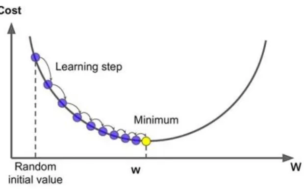
The core of the gradient descent algorithm is to move in the direction of the steepest drop of the loss function each time, and the steepest direction is usually the opposite direction of the vector obtained by taking the partial derivative of the loss function with respect to the weight vector.

(27)

In order to calculate the above vectors, we calculate each component one by one:

Formula 9

Each weight update is:

Formula 10

The weight updating method using this method is called gradient descent, which calculates a sum of all training centralization values and then updates the weight. This method needs to train all the training sets once to update the sequential weights, so it is slow and inefficient.

To improve this slow updating speed, the stochastic gradient descent algorithm is adopted, and the weight vector updating formula is:

Formula 11

The above algorithm is generally applied to each neuron in all types of neural network models. After understanding the role of each neuron, it is necessary to mention the key algorithm that makes the neural network play a role, the back-propagation algorithm.

(28)

Figure 3 An example of gradient descent

3.1.2 Back-propagation algorithm

Neural network is to take a single perceptron as a neural network node, and then use such nodes to form a hierarchical network structure; we call this network as artificial neural network. When the number of layers of a network is greater than or equal to 3, we call it a multilayer neural network or Multi-Layer Perceptron (MLPs).

In the previous section, we introduced the perceptron algorithm, but there are the following problems in direct use:

1) Output of perceptron training rules:

Formula 12

Since the sign function is non-continuous, which makes it non-differentiable, the gradient descent algorithm above cannot be used to minimize the loss function.

2) The output of delta rule:

(29)

Formula 13

Each output is a linear combination of inputs, so that when multiple linear units are connected together, only linear combinations of inputs can be obtained eventually, which is not very different from having only one perceptron unit node.

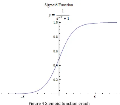
In order to solve the above problems, on the one hand, we cannot directly use the linear combination of direct output, need to add a processing function when the output; On the other hand, the added handler must be differentiable so that we can use the gradient descent algorithm. There are many functions that satisfy the above conditions, but the most classic one is sigmoid function, also known as Logistic function, which can compress any number within to between (0,1), so this function is also known as the extrusion function. In order to normalize the input of this function, we add a threshold value to the linear combination of the input, making the linear combination of the input 0 as the cut-off point.

Formula 14 the sigmoid function

(30)

This function has an important property which is its derivative:

Formula 15 the derivative of sigmoid function

And it makes it a lot easier to calculate the gradient descent.

In addition, the tanh function can also be used to replace the sigmoid function. The curves of the two functions are similar.

Formula 16 the derivative of tanh function

The processing of Back-propagation algorithm which in feed forward network with two-layer sigmoid unit:

1) Randomly initialize the ownership value in the network. 2) For each training sample, perform the following operations:

A) Calculate from front to back according to the input of the instance to obtain the output of each unit of the output layer.

The error term of each unit in each layer is then calculated in reverse from the output layer.

B) For each unit k in the output layer, calculate its error term:

Formula 17

C) For each hidden unit h in the network, calculate its error term:

Formula 18

(31)

Formula 19

Formula 20

In this processing, X𝑗𝑖is input of node i to node j, and w𝑗𝑖 stands the corresponding

weight. Outputs mean the represents a collection of output layer nodes. In this experiment, all the models I used will adopt similar neurons and gradient optimization methods.

3.2 Embedding representation

3.2.1 Word2vec

Before word2vec, there was no simple way to represent a text in NLP. From one-hot encoding represents a word to using BoW to represent a piece of text, the author used k-shingles to divide text into text segments, and The author using various sequence annotation methods to segment text semantically, in tf-idf, the author using the frequency of words to represent the importance of words, to in the text-rank [12] reference page-rank method to represent the weights of words, the author based on SVD decomposition of matrix which is LSA [13], In pLSA[14], the process of document formation is represented by means of probability and the solution result of word document matrix is endowed with probability meaning. In LDA, two conjugate distributions are introduced to perfectly introduce the prior.

However, the understanding of deep semantics is not satisfactory. It's often assumed that methods like word2vec give each word a vector representation, but no one seems to

(32)

have thought before about why this works. In theory, the main starting point of these methods, including NNLM [15], is to represent a word as a word vector and represent its semantics through context. In fact, there is a theoretical basis behind it. Harris proposed the distributional hypothesis in 1954. It holds that words with similar contexts also have similar semantics. The semantics of words are determined by their context (a word is characterized by the company it keeps), and 30 years later, Hinton, the grandfather of deep learning, tried the distributed representation of words in 1986. The contribution of word2vec is not only to give each word a distributed representation, but also to bring a new NLP modeling method. Prior to this, most NLP tasks spent a lot of time on how to explore more semantic features of text, and even this part of the work accounted for the majority of the workload of the whole task.

Word2vec for the former optimization, mainly two aspects of work: model simplification and training skills optimization. For the simplification of the model, there are some classical models known as the CBOW and Skip gram [15].

Formula 21 objective function of CBOW

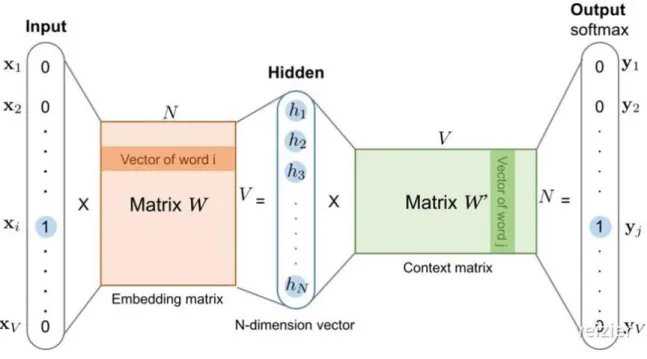
CBOW didn’t have any hide layer, essentially only two layer structure, the input layer’s function is to calculate the vectors of every word in target word’s context C for simple summation (or average), and then dot product with the target word’s vector directly. the objective function is to get the max value of dot product, and at the same time, to get the min value which is the dot product between context C and other non-target word.

(33)

NNLM and directly connects the input layer with the output layer; The second is that the word order in context is discarded when the context vector is calculated; Third, the final objective function is still the objective function of the language model, so each word in the corpus needs to be traversed sequentially. With these characteristics, for this simple but effective model, Mikolov named this simple model the CBOW.

Figure 5 the structure of CBOW

It is important to note here every word vector corresponding to the two words, are reflected in the above formula, 𝑒(𝑤_𝑡) is a input vector of word, and 𝑒′_(𝑤

𝑡) is a output

vector of word, or more accurately, the former is CBOW input layer and connected all the word 𝑤_𝑡 are located in the edge of the weight, vector instead of in the output layer are connected to the location in which the word 𝑤_𝑡 variegated weight vector Similarly, corresponding to the CBOW, Skip gram's basic idea of the model is very similar to the CBOW, only in a different direction: the CBOW is the vector x that makes the output vector 𝑒′_(𝑤

(34)

each word in the context try to fit the vector 𝑒(𝑤_𝑡) of the current input word, which is opposite to the direction of CBOW, so its objective function is as follows:

Formula 22 objective function of Skip-gram

It can be seen that there are two summation symbols in the target function, and the meaning of the summation symbol in the innermost part is to make the current input word as close as possible to each word in the corresponding context of the word, so as to show that the word is as close as possible to its context.

(35)

Similar to the CBOW, Skip-gram essentially has only two layers: input layer and output layer. The input layer is responsible for mapping the input word into a word vector, and the output layer is responsible for calculating the probability of each word through linear mapping. In fact, both the CBOW and skip-gram are essentially two fully connected layers connected without any other layers in between. As a result, the number of the parameters of the two models are 2 ∗ | e | ∗ | V |, which | e | and | V | respectively is the size of the word vector dimension and dictionaries.

Mikolov mentioned the Hierachical Softmax in the article at first, thinking as an optimization method of full Softmax, and the Hierachical Softmax basic idea is: Firstly, every word from the corpus, in accordance with the word size to construct a Huffman tree, guarantee the words with high frequency in a relatively shallow layer, low frequency words are relatively deep Huffman tree leaf nodes, Each word is on a leaf node on this Huffman tree.

Secondly, the original | V | classification problem was changed into the binary classification problem of log | V | . When they originally calculated P(w_𝑡|c_𝑡), since they used ordinary softmax, they had to ask the probability of each word in the dictionary. In order to reduce the calculation, the Hierachical Softmax was be used, the corresponding is a binary classification problem, It is essentially a linear regression classifier, and the construction process of Huffman tree guarantees that the depth of the tree is log | V | , so it only needs to do log | V | binary classification to get the size of P(w𝑡|c𝑡), which is

greatly reduced compared to the original calculation of | V |.

Then Mikolov proposed the idea of negative samples, and this idea is also inspired by the C&W model structure of negative sample method, and the reference Noise Contrastive Estimation (an NCE) thought, with CBOW simply is, the framework of negative sample each traversal to a target word, in order to make the target word probability P(w_𝑡|c_𝑡) is the most, according to the probability formula of softmax function, also is to make the molecules of the biggest, and other non-target word minimum in the denominator.

(36)

The calculation of ordinary softmax is too heavy because it takes all other non-target words in the dictionary as negative examples, and the idea of negative sampling is very simple, that is, every time random sampling some words according to a certain probability as negative examples, so you only need to calculate the negative examples of these negative samples, then the probability formula will be:

Formula 23 target word probability of word2vec

Careful comparison with ordinary softmax shows that the original |V| classification problem is changed into a K classification problem, which turns the effect of dictionary size on time complexity into a constant term, and the change is very small, which is subtle.In addition; Mikolov also mentioned some other techniques. For example, for words with ultra-high frequency, especially stop words can be processed using Subsampling method. However, this is not the main content of word2vec.

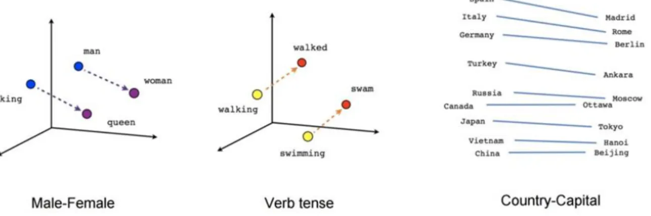
Since then, through the double optimization of model and training skills, the training on large-scale corpus has finally become a reality. More importantly, the obtained word vectors can have a very good semantic performance and can represent the semantic relationship through the vector space.

(37)

Word2vec, greatly promoted the development of NLP, especially to promote the application of deep learning in NLP, pre trained word vector is used to initialize the first layer of the network structure has almost become the standard, especially in the case of only a small amount of training data.

3.3 Model

3.3.1 Multi-Layer Perceptron

MLPs is derived from the Perceptron Learning Algorithm (PLA). The most important feature of MLPs is that there are multiple layers of neurons, so it is also called DNN (Deep Neural Networks).And as shown in the figure:

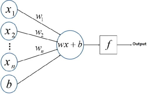
Figure 8 the network topology of single neural unit

Assume that the input space is 𝑋 ⊆ 𝑅_𝑛, of which the characteristic vector 𝑥 ∈ 𝑋; The output space is 𝑌 = *+1, 1+, and the output is 𝑌.

(38)

Formula 24

𝑋_𝑖 is the input value, 𝑊_𝑖 stands the weight corresponding to each input 𝑋_𝑖, 𝑏 is the bias, and 𝑠𝑖𝑔𝑛 is the activation function.

Geometric interpretation of the perceptron model: the linear equation 𝑤 ∙ 𝑥 + 𝑏 = 0 corresponds to a hyperplane 𝑺 in the eigenspace 𝑅_𝑛, where w is the normal vector for the plane and b is the intercept for the hyperplane. The hyperplane divides the space into two parts, instances in different parts belong to different categories, and instances in the same part belong to the same category.

Suppose there is a hyperplane, which can perfectly separate the instances in the data set so that different types of instances belong to both sides of the hyperplane, then the data set is said to be linearly separable. For linearly separable datasets, the perceptron model looks for a hyperplane that perfectly separates the dataset. The hyperplane is determined by the parameters w and b.

To find the appropriate parameters, you need to specify a policy that defines and minimizes the empirical loss function. Loss function can naturally select the total number of instances separated by loss, but it is not recommended because it is not conducive to optimization. So it's the distance from the instance to the hyperplane. The perceptron learning problem is to find an appropriate model in the hypothesis space. The problem then becomes an optimization problem that minimizes the empirical risk.

It can be seen from the above content that PLA is a linear binary classifier, but it cannot effectively classify non-linear data. Therefore, with the deepening of network layer, an important feature of multi-layer perceptron is multi-layer. We call the first layer as input layer, the last layer as output layer, and the middle layer as hidden layer.

(39)

MLPS do not specify the number of hidden layers, so you can choose the appropriate number of hidden layers according to your needs.

There is no limit to the number of neurons in the output layer. In theory, a multilayer network including at least one hidden layer can simulate any complex function.

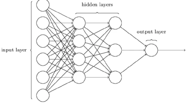
From the perspective of neural network, MLP is also called multi-layer neural network, and its network structure is as follows:

Figure 9 network structure of MLPs

In the feed-forward neural network, the information only moves one item, that is, it moves forward from the input layer, then through the hidden layer, and then to the output layer. There is no loop in the network.

As we know, the core of neural network algorithm is to define and minimize the loss function.

In order to minimize the loss function, we will train our multilayer perceptron, and training method is the back propagation algorithm, we have been in the last section, the back propagation algorithm is one of several ways of training the neural network, this is a method of supervised learning is learning by labeled training data.

(40)

3.3.2 Convolutional neural networks

Convolutional neural networks (CNN) belong to the category of neural networks, and such network structure and variant structure are now widely used in the field of image processing. Many researchers have made breakthroughs in this direction, and such fields as image recognition and classification have proved their efficient ability. Now, convolutional neural networks can successfully recognize faces, objects and traffic signals to provide vision for robots and self-driving cars.

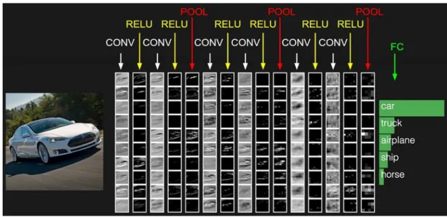
Figure 10 An example of the application of convolutional neural networks in the image classification

LeNet is one of the earliest convolutional neural networks to promote the development of deep learning. After several successful iterations, by 1988, Yann LeCun named the pioneering work LeNet5 [16]. At that time, LeNet architecture was mainly used for character recognition tasks, such as reading zip codes, Numbers and so on.

It seems that the most suitable job for CNN is classification task, such as emotion analysis, spam identification or subject classification. But Convolutions and Pooling operation will ignore the local information of word order, this makes in the task of sequence annotation like part-of-speech tagging or named entity recognition, is too difficult to use just CNN architecture.

(41)

researchers have proved that CNN can have very good effect on text classification task, in [17], they used various categories of corpus (mostly sentiment analysis and subject classification task), to verify a CNN model, and CNN model in all the corpus shows great effect, and in several corpus, CNN model get the highest accuracy.

Surprisingly, the network used in the paper is quite simple, which is what makes it powerful. I think the advantage is good at dealing with deep learning "intensive", "relevant" data, no matter image data or text data, there are strong dependencies, but there is also a strong redundancy, if we just dropout a small piece of word in a text, to our understanding of the image and text is not much affected. So we can extract the features of compressed images through CNN.

Many researchers have also done related studies. For example, [18] instead of pretraining word vectors like word2vec or GloVe, a CNN was trained from 0. He applied the one-hot vector directly to the convolution layer. the author also puts forward an expression similar to BOW as the input of data to reduce the number of parameters that need to be learned in the network and improve the utilization rate of space.

[19] attempted to use CNNs for relationship extraction task and relationship classification task. In addition to using the word vector. The model assumes that the position of the entity word is given, and that each sample input contains a relationship.

Figure 11 the structure of sentiment analysis

As shown in the figure above the structure of the CNN model is as follows:

(42)

word2vec, we can transform word into vector, and put the words in order, finally we can get the sequence of a sentence.

Convolution layer, Convolutional neural networks in each layer convolution is

composed of several convolution unit, parameters of each unit are obtained by back propagation algorithm. The purpose of convolution operation is to extract different features of input. The first convolutional layer may only extract some low-level features. The multi-layer network can iteratively extract more complex features from low-level features.

Pooling layer obtains the features with large dimensions after the convolution layer.

Cut the features into several areas and take the maximum or average value to obtain the new features with low dimensions.

Fully Connected layer, which combines all local features into a global feature, is used

to calculate the score of each category.

3.3.3 Recurrent neural network

Whether it is a convolutional neural network or an artificial neural network, their premise is that the elements are independent of each other and the input and output are also independent, such as cats and dogs. But in the real world, many elements are interconnected, such as the change of stocks over time. One person said:” I like traveling, and my favorite place is Kyoto. I will go to ___ if I have chance”. Because we are inferring from the context, but the opportunity to do this step is quite difficult.

So, with the recurrent neural network (RNN) [20] that we have today, it's essentially: the ability to remember like a person. Therefore, its output depends on the current input and memory.

Recurrent neural network is on the basis of ordinary multi-layer BP neural network, increase the horizontal linkages between the hidden layer units, with a weight matrix, can be on a time series of neural unit value passed to the nerve cell, so that the neural network

(43)

has the memory function, for processing a context of NLP, or time series machine learning problem, has a good applicability.

In this study, RNN structure is not adopted, but LSTM is a variant of RNN. Before understanding the algorithm flow of LSTM, we need to first understand the algorithm flow of RNN. The figure below is the algorithm flow of RNN:

Figure 12 the structure of RNN

As shown in the figure above, we define 𝑋_𝑡 as the input at time t, 𝑜𝑡 as the output at

time t, 𝑆𝑡 as the memory at time t, there are:

𝑜𝑡 = 𝑠𝑜𝑓𝑡𝑚𝑎𝑥(𝑉 ∗ 𝑆𝑡)

Formula 25

Formula 25 is the calculation formula of the output layer. The output layer is a full connection layer, which is each node of it is connected to each node of the hidden layer. V is the weight matrix of the output layer, and softmax is the activation function.

𝑆_𝑡= 𝑓(𝑈 ∗ X_𝑡+ 𝑊 ∗ S_𝑡−1)

Formula 26

Formula 26 is the calculation formula of hidden layer, which is the recurrent layer. U is the weight matrix for the input x, W is the last value as the weight matrix for the input this time t, and f is the activation function.

(44)

This is a basic RNN model. The reason why the RNN model can reflect the

characteristics of sequential data is that each 𝑆_𝑡 retains part of the 𝑆_𝑡−1 information, and this structure ensures that part of the information in the text will be retained, thus

reflecting the characteristics of timing.

RNN has the advantage of being able to memorize the model, but it also has the defect which cannot memorize the contents of the former or the latter, because of gradient explosion or gradient disappearance.

LSTM and bidirectional LSTM, which will be introduced in the next section, can not only preserve the temporal features in sentences, but also avoid the loss of semantic relations in long sentences.

3.3.4 LSTM

Long short term memory [21], also known as LSTM, is specially designed to solve long-distance dependency problems. All RNN have a chain form of repeating neural network modules. In standard RNN, this repeating structure module has only a very simple structure, such as a tanh layer.

Figure 13 the tanh layer in RNN unit

The LSTM has the same structure, but repeated modules have a different structure. Instead of a single neural network layer, there are four, interacting in a very specific way.

(45)

Figure 14 the structure of LSTM

In the illustration above, each black line transmits an entire vector from the output of one node to the input of another node. The pink circles represent pointwise operations, such as vector sums, while the yellow matrix is the layer of learned neural networks. The combined lines represent concatenation of vectors, and the separate lines indicate that the content is copied and distributed to different locations.

The core idea

The whole green diagram is a cell, and the key to LSTM is the state of the cell, and the horizontal line across the cell.

(46)

The cell state is like a conveyor belt. It runs directly through the chain, with only a few linear interactions. It would be easy for information to circulate and stay the same.

Figure 16 activation operation

We cannot add or remove information with only the horizontal line above. So it's done through a structure called gates. Gates allow information to pass selectively, primarily through a neural layer, in fig.15, σ stands activation function operation and the pink circle stands an element wise multiplication operation.

Each element of the sigmoid layer output (which is a vector) is a real number between 0 and 1, representing the weight (or proportion) through which the corresponding information passes. For example, 0 means "don't let any information pass" and 1 means "let all information pass".

The LSTM implements the protection and control of information through three such structures. The three gates are the input gate, the forgetting gate and the output gate.

Forget gate

The first step in our LSTM is to determine what information we discard from the cell state. This decision is made through a layer called the forget gate. The gate will get 𝑕𝑡−1 ,

𝑥𝑡 and outputs a value between 0 and 1 to each number in the cell state 𝐶𝑡−1. 1 means

(47)

Figure 17 forget gate

Input gate

The next step is to decide how much new information to add to the cell state.

There are two steps to implementing this: first, an input gate layer called sigmoid determines which information needs to be updated;

A tanh layer to generate a vector, which is optional used to update the content of 𝐶̃𝑡.

Figure 18 input gate

In the next step, combine the two parts to make an update to the status of the cell. 𝐶_𝑡−1 was updated to 𝐶_𝑡. We multiply the old states by 𝑓_𝑡 and discard the information that we want to dropout, then add 𝑖_𝑡∗ 𝐶̃_𝑡. These are the new candidate values, varying according to the degree to which we decide to update each state.

(48)

Figure 19 updating the state of cell 𝐶𝑡

Output gate

Finally, we need to determine what the output is. This output will be based on our cell state, but it is also a filtered version. First, we run a sigmoid layer to determine which parts of the cell state will be exported. Next, we process the cell state through tanh (to get a value between -1 and 1) and multiply it by the output of the sigmoid gate, and in the end we will only output what we have identified as the output.

Figure 20 output gate

LSTMs are explicitly designed to avoid the long-term dependency problem. Remembering information for long periods of time is practically their default behavior. LSTM networks have the form of a chain of repeating modules of neural network.

3.3.4.(i) Bi-LSTM

The ability to access future context as well as past context information is beneficial for many sequence annotation tasks. For example, in the most special character sorting, it

(49)

would be very helpful to know what letter is coming, just as it was before the letter. The basic idea of Bi-LSTM is to propose that each training sequence is two LSTM forward and backward respectively, and both of them are connected with an output layer. This structure provides the output layer with complete past and future context information for each point in the input sequence. The figure below shows a bidirectional LSTM that unfolds over time.

Figure 21 the structure of Bi-LSTM

Six unique weights are repeatedly utilized in each time step, corresponding to six weights respectively: input to forward and backward hidden layer (w1, w3), hidden layer to hidden layer itself (w2, w5), forward and backward hidden layer to output layer (w4, w6). And there is no information flow between the forward and backward hidden layers, which ensures that the expansion diagram is non-cyclic.

(50)

3.4 Attention mechanism

The mechanism of Attention was first proposed in the field of Visual images in the 1990s. It is believed that the core idea has been proposed, but it is the “Recurrent Models of Visual attention [22]” published by the Google mind team that has a rising popularity. Subsequently, Bahdanau et al. in their paper "Neural Machine Translation by understanding Learning to Align and Translate" [23] used a mechanism similar to attention to simultaneously Translate and Align in Machine Translation tasks, and their work is the first one to propose the application of the attention mechanism to the NLP field. Then a similar RNN model extension based on the attention mechanism was applied to various NLP tasks. Recently, how to use the attention mechanism in CNN has become a research hotspot. The chart below shows the broad trends in research progress in attention.

3.4.1 Global Attention and Local Attention

Luong et al. [24] proposed Global Attention and Local Attention. Global Attention is essentially similar to Bahdanau et al. [13].

The Global method, as its name implies, looks at all the words in the sequence of source sentences, specifically taking into account all the hidden states of the encoder when calculating the semantic vector.

However, in Local Attention, the computation of semantic vector only pays Attention to a part of the hidden state of the encoder of each target word.

Since the Global method must calculate all the hidden states of the source sentence sequence, long sentences can be expensive to calculate and make translation impractical, such as when translating paragraphs and documents.

(51)

(52)

3.4.2 Attention model in this study

Figure 23 shown the structure of attention layer

In this figure, 𝑕_𝑡𝑠 stand the Sth hidden state on time t , and the 𝑎𝑡 stands the global

weight, and the 𝐶_𝑡 is the context vectors, and for 𝑕_𝑡𝑠_{. The}_𝑎

𝑡 is an alignment vector of

variable length, which is equal to the length of the input part time series.

𝑎𝑡(𝑠) is obtained by comparing the current hidden layer state 𝑕𝑡𝑠 with the state 𝑕𝑡𝑚 of

each hidden layer:

𝑎_𝑡(𝑠) = 𝑎𝑙𝑖𝑔𝑛(𝑕_𝑡𝑚_{, 𝑕} 𝑡𝑠)

(53)

= exp (𝑠𝑐𝑜𝑟𝑒(𝑕𝑡 𝑚_{, 𝑕} 𝑡𝑠)) ∑ exp (𝑠𝑐𝑜𝑟𝑒(𝑕_𝑡𝑚_{, 𝑕} 𝑡𝑠 ′ )) 𝑠′ Formula 27

Score is a content-based function, which can be implemented by the method below: 𝑠𝑐𝑜𝑟𝑒(𝑕_𝑡𝑚, 𝑕_𝑡𝑠) = 𝑕_𝑡𝑚⊺_𝑊

𝑎𝑕𝑡𝑠

Formula 28

By integrating all the 𝑎_𝑡(𝑠) into a weight matrix, 𝑊𝑎 is obtained, which can be

calculated as:

𝑎_𝑡= 𝑠𝑜𝑓𝑡𝑚𝑎𝑥(𝑊_𝑎𝑕_𝑡)

Formula 29

By doing a weighted average operation on 𝑎_𝑡, then we can get context vector 𝐶_𝑡. 𝐶_𝑡 and 𝑕_𝑡𝑚 were spliced and input into the classifier. Finally, the weight of 𝑎_𝑡 was adjusted by the back-propagation algorithm.

(54)

Chapter 4

Experiment

4.1 Dataset

In this study, I used dataset from SemEval-2014 Task4, there is two domain-specific datasets for laptops and restaurants, consisting of over 6K sentences with fine-grained aspect-level human annotations have been provided for training.

Figure 24 the sample of datasets

Restaurant reviews dataset consists of over 3K English sentences from the restaurant reviews of Ganu et al. [25]. The original dataset of Ganu et al. included annotations for coarse aspect categories and overall sentence polarities; I modified the dataset to just include polarities of the reviews. I also corrected some errors (e.g., sentence splitting errors) of the original dataset. Experienced human annotators identified the aspect terms of the sentences and their polarities. Additional restaurant reviews, not in the original dataset of Ganu et al. [25], are being annotated in the same manner, and they will be used as test data. And the laptop reviews dataset consists of over 3K English sentences extracted from customer reviews of laptops. Experienced human annotators tagged the aspect terms of the sentences and their polarities.

4.2 Word Embedding

(55)

punctuation from the participle list.

The maximum length of the text after processing is 70.

In order to construct the feature vector, the word vector has a dimension of 300, and the word vector is initialized in two ways:

(1) Random initialization: all words are randomly initialized and word vectors are

dynamically updated in the training process.

(2) Using the word2vec: use the open source tool word2vec proposed by Google in

2013 to train the word vector. At the same time, randomly initialize the words that do not appear, and dynamically update the word vector in the training process.

4.3 Hyper-parameter Settings

For all the models the epoch is 20, and the batch size is 64, and the setting of model parameters is very important. The main parameters in the model are set as follows:

Model name Initialization method Attention MLPs Random MLPs Word2vec CNN Random CNN Word2vec LSTM Random Without With attention LSTM Word2vec Without With attention

(56)

With attention

Bi-LSTM Word2vec Without

With attention Chart 1 Structures of all experiments

For the MLPs, the hyper-parameter setting is as follow:

name Hidden layer Unit

MLPs640 2 320+320

MLPs1280 3 320+640+320

MLPs2560 4 320+1280+640+320

Chart 2 Structures of each MLPs

For each hidden layers, I set dropout parameter in 0.2

For the CNN, the hyper-parameter setting is as follow:

name convolution layer Unit

CNN600 2 300+300

CNN900 3 300+300+300

CNN1200 4 300+300+300+300

Chart 3 Structures of each CNN

For each model of CNN, there is a pooling layer behind convolution layer, and the pooling method is max pooling, and the final layer is a full connection layer and the dropout is 0.2.

For the LSTM, the hyper-parameter setting is as follow:

(57)

LSTM64 64

LSTM128 128

LSTM256 256

Chart 4 Structures of each LSTM

The final layer is a full connection layer and the dropout is 0.2.

For the Bi-LSTM, the hyper-parameter setting is as follow:

name Unit

Bi-LSTM64 64

Bi-LSTM128 128

Bi-LSTM256 256

Chart 5 Structures of each Bi-LSTM

The final layer also is a full connection layer and the dropout is 0.2.

4.4 The LSTM with Attention Model

(58)

Figure 25 the structure of Bi-LSTM with Attention Model

As shown in fig.23, 𝑊_𝑡1_{, 𝑊}

𝑡2, 𝑊𝑡𝑚stand the vectors of each word in sentence, and the

𝑕𝑡1, 𝑕𝑡2, 𝑕𝑡𝑚stand the state of each vector in the processing of Bi-LSTM, after feed forward

of Bi-LSTM, by using the BP algorithm, we can get the weight in attention layer and the weight of Bi-LSTM unit. Finally Until converges, we get the trained model.

JAIST Repository: A Study on Long-Short Term Memory Networks with Attention Mechanism