JAIST Repository: Adaptive Routing Protocol for Multiple Portal in Wireless Mesh Networks

(1)

JAIST Repository

https://dspace.jaist.ac.jp/

Title Adaptive Routing Protocol for Multiple Portal in Wireless Mesh Networks

Author(s) 陳, 鑽

Citation

Issue Date 2013-06

Type Thesis or Dissertation Text version author

URL http://hdl.handle.net/10119/11399 Rights

Description Supervisor:Lim, Azman Osman, School of Information Science, Master

(2)

Adaptive Routing Protocol for Multiple Portal in

Wireless Mesh Networks

By CHEN Zuan

A thesis submitted to

School of Information Science,

Japan Advanced Institute of Science and Technology,

in partial fulfillment of the requirements

for the degree of

Master of Information Science

Graduate Program in Information Science

Written under the direction of

Associate Professor LIM Azman Osman

(3)

Adaptive Routing Protocol for Multiple Portal in

Wireless Mesh Networks

By CHEN Zuan (1110041)

A thesis submitted to

School of Information Science,

Japan Advanced Institute of Science and Technology,

in partial fulfillment of the requirements

for the degree of

Master of Information Science

Graduate Program in Information Science

Written under the direction of

Associate Professor LIM Azman Osman

and approved by

Associate Professor LIM Azman Osman

Professor TAN Yasuo

Professor SHINODA Yoichi

May, 2013 (Submitted)

(4)

Acknowledgements

First and foremost, I would like to thank my supervisor, Associate Professor Lim Azman Osman, for the patient guidance, encouragement and advice he has provided throughout my time as his student. I have been extremely lucky to have a supervisor who cared so much about my research and my life.

I would also like to thank all the members in Tan, Lim, Shinoda and Chinen Labora-tories in JAIST for their kindness to give their supports for my research.

In particular I would like to thank Professor Tan Yasuo, my sub supervisor for his suggestions and support throughout my research studies.

I would also like to specially thank Professor Shinoda Yoichi. Thanks him for his com-ments on my research.

Finally I would like to thank my mother for her unconditional support, both ﬁnancially and emotionally throughout my life in Japan.

(5)

Chapter 1 Introduction

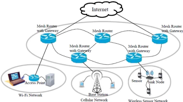
Wireless mesh network (WMN) is a type of communication networks that construct by radio nodes in a mesh topology. The WMN typically consist of mesh routers, mesh clients and gateways. The mesh routers are used to forward packets on behalf of other nodes that are out of direct transmission range of their destinations and may also act as gateway in mesh routers to integrate the WMNs with others existing wireless networks such as wireless sensor networks, cellular systems, wireless-ﬁdelity (Wi-Fi), worldwide inter-operability for microwave access (WiMAX), etc. Whereas the mesh clients are elec-tronic communication devices such as laptop, desktop, cell phone, PocketPC, etc. Fig. 1.1 shows the WMN structure.

(8)

In WMN, the nodes are able to establishing and maintaining their connectivity among themselves, which means, they are dynamically self organized and self-conﬁguration. Due to these features, the network providers are able to change, expand, and adapt the network as needed to meet the demands of the end users. Therefore, WMN are getting popular in the upcoming communication technology especially when it provides a promising wireless technology for numerous applications, e.g., broadband home networking, community and neighbourhood networking, building automation, etc.

Moreover, the mesh routers in the WMN have the ability to service in multi-hop envi-ronments. Hence, the uses of wireless routers in large areas are cheaper than the single hop routers in wired connections. The wired connections require installation and maintenance that are more expensive, while the WMN deployment with easier and fast installation and maintenance that leads to lower operation cost. In addition, there are multiple paths from the source to destination in the WMN. Thus, it provides an alternative path for the case of link failure and bottlenecks point to mitigate the congestion in the networks. This feature also allows the traffic loads to be balanced in the networks and significantly increase network reliability in WMN. In the traditional wireless networks, the number of nodes is inversely proportional to the network performance. When the number of nodes is increased, the network performance will be descendent. However in the WMN, when the number of nodes is increased, the transmission capacity will also increase and give a better load balancing and alternative routes. Usually, the local packets are run faster than the packets from the neighbours. This is mainly due to the some WMN configurations and protocol that manage the communication medium.

In the following section, we will discuss the application of WMN, research scope and problem, and the background study. At the background study part, we focus on the ar-chitecture of WMN, airtime link metric, and hybrid wireless mesh network. The chapter will end with the thesis outline description.

1.1 Application of WMN

The features of WMN allow it to fully support some applications that cannot be im-plemented by other wireless technologies. For instances the applications in broadband wireless access, industrial applications, healthcare, warehouse, transportation systems, hospitality, etc. Currently, broadband access plays an important role in an information economy. It provides services for real time applications such as video streaming, online gaming, teleconferencing, etc. In order to widely adoption of internet access even in ru-ral areas, the WMN will be the best choice because it oﬀers an easy-to-deploy and cost eﬀective alternative in areas where cable TV or DSL lines are not available. Although the satellite and cellular network are able to provide the same service as WMN, they are an expensive technology and high latency due to the distance between end client and the satellite or cellular.

In the industrial application especially building automation, there need many devices to monitor and control the building environment, for instances the electrical power, light, air conditioner, elevator, etc. The wired network and Wi-Fi network are currently used to

(9)

taking care such environment, but the deployment of wired network will increase the net-work complexity whereas Wi-Fi netnet-work solution will increase the cost due to expensive wiring Ethernet for Wi-Fi access point. However, if the Wi-Fi access point is replaced by mesh routers, the deployment process will become simpler and the cost can be reduced signiﬁcantly.

In the healthcare applications, the patient information in hospital or medical centre such as medical history, test results, insurance information, etc., need to be processed and transmitted from room to room for monitoring and updating. Therefore, they need the network that able for data access in every operating room, office and laboratory, and transfer a large amount of data due to high resolution medical images and periodical monitoring information. The WMN is able to provide an unlimited network access to any fixed medical devices, and it does not need to use existed Ethernet connections. Thus, the dead spots problem can be eliminated. Whereas the warehouses applications, they need the connectivity throughout the area to keep track of stock by handheld scanner. Therefore, the WMN will be the best suit since it can ensure the connectivity in modern warehouses and shipping logistics with little cost and effort.

In order to extend the internet access from the stations to each destination stops for the public transportation system such as busses, plains, trains and ferries, WMN technology can give a well support. In addition, WMN is also sustenance to the remote monitor-ing in-vehicle, driver communications and security cameras in the transportation system. Meanwhile, the hospitality application such as high-speed Internet connectivity in the ho-tels and resort by implementing the WMN can easier the network set up, reduce the cost, and maintain the existing structures or disrupt business for both indoor and outdoor.

1.2 Research Scope and Problem

The architecture of WMN that builds within the MAC layer of IEEE802.11 devices is specified in the IEEE802.11s standard. In IEEE802.11s standard, several aspects of the basic specification are introduced. For example, (i) it specifies new frame formats and information elements; (ii) it presents the path selection and forwarding procedures; (iii) it supports non-mesh stations by means of proxy operations; (iv) it adopts a new security framework to the mesh architecture; and (v) it states the peer node discovery and the management of the established link.

Among all these aspects, one of the most features is the path selection procedure, which is based on the Hybrid Wireless Mesh Protocol (HWMP). HWMP forms multihop paths that connect the mesh stations. This operation is accomplished by means of the airtime link metric (ALM), a newly specified metric that tries to capture the quality of the links as a function of the estimated frame loss probability. Because of these considerations, it is lead us to investigate the implementation and efficiency of the HWMP and the ALM. In our research studies, the original ALM value is not a suitable one for calculating and identifying short distance transmission. To address this problem, we propose a modified link metric which is comfortable for distinguishing different distance wireless transmis-sions.

(10)

In additions, we face traﬃc balancing problem for the existence of multiple portal in WMNs, especially in the uplink transmission. In uplink, mesh access point (MAP) or mesh point (MP) sends, or uploads data packets to the mesh portal point (MPP). In this context, MAP is used to support WLAN services, which allow them to help other nodes to transmit packets, meanwhile extend the wireless transmission range. The MPP are MAP which provides connectivity to other networks. In order to resolve this problem, we proposed an adaptive routing protocol with traﬃc balancing algorithm for multihop WMNs.

For the data transmission through the MPP, we also face the problem that we need to apply any Address Resolution Protocol (ARP) in our proposed protocol to discover the MAC address in the data link layer in between Internet and WMNs. In our research, we are not focused on proposing the ARP protocol. We assume that our proposed protocol uses embedded ARP to solve the addressing problem.

1.3 Related Work

A few research work concerning the problem of traffic balancing for multiple mesh gate-way in the WMNs. Tao et al. show how traffic balancing (TB) method solves the uneven traffic load problem appearing in WMNs. With the right placement of the mesh gateway, TB method can improve the performance of routing protocol dramatically. Maurina et al. introduce a tree-based with multi-gateway association (TBMGA), a novel routing protocol that elegantly balances the load among the different Internet gateways in the WMNs. TBMGA combines the flexibility of layer-2 routing with the self-configuring and self-healing capabilities of mobile ad hoc network (MANET) routing. The selection of gateway is depending on a global metric estimated based on the average queue length and expected availability at the Internet gateway. Galvez et al. study a feedback-based adap-tive online algorithm for multi-gateway load-balancing in the WMNs. The algorithm is called gateway load-balancer (GWLB), which executes periodically, adapting to network conditions. GWLB takes into account the elastic nature of TCP flows, as well as flow interactions when switching nodes between domains, in order to prevent severe interfer-ence. Ashraf et al. propose expected link performance-gateway selection (ELP-GS), which is used to handle gateway and route selection for gateway-oriented traffic. Along with ELP-GS, they also propose a gateway discovery protocol to help evaluate the extended ELP metric at finding the ‘best’ available route between mesh routers for peer-to-peer traffic. Owing to selection of ‘best’ routes to the gateway along with the least loaded gateway, overall ELP-GS provides better throughput, lower end-to-end delay and lower delay-deviation.

1.4 Research Motivation

Up to date, many researchers were doing the research on the traﬃc balancing prob-lem for multiple portal in WMNs, they focused on diﬀerent points of view according to

(11)

the existing researches and publications. However, the project of IEEE802.11s was also working on the way, and ﬁnally published a release version on September 2011, coming from IEEE802.11s Draft #12 which met with 97.2% approval rate. On the related works, researchers didn’t do their researches based on the IEEE802.11s mesh networking. On the other hand, none of these researchers had studied the latency as routing metric in WMNs. Latency is also an evaluation point for the performance of WMNs. In IEEE802.11s, air-time link metric (ALM) was proposed as default metric to measure the airair-time cost in WMNs. ALM is a radio-aware metric compared with metrics in Wired Network. Hence, we also need to studies ALM.

Motivated by these facts, our research aims to propose a routing protocol using optimal load balancing algorithm to balance the traﬃc load for multiple portal in WMNs which is under the IEEE802.11s mesh networking. We use both ALM and latency as routing metrics to do the traﬃc balancing in WMNs, and we also evaluate the performance of our proposed algorithm by simulations.

1.5 Thesis Outline

Chapter 2 introduces a brief review of WMN and IEEE 802.11s standard of Mesh Networking, which include the features and functions. It also highlights the routing that used the ALM to capture the quality of the links as a function of the estimated frame loss probability. Then, the performance evaluation based on ALM performance, single MPP, multiple MPPs using ALM and setting, parameters are described. The simulation results are also deeply discussed in the chapter.

Chapter 3 describes the network model and assumptions in our research, the problem to be solved and proposes our traffic balancing algorithm for multiple portal, which is called Optimal Latency Balancing Algorithm. In this chapter, we also evaluate and study the performance of the proposed algorithm by seting up the simulation environment, defining the different scenarios and discusses the results of our proposed algorithm accordingly with scientific factors and reasons.

Chapter 4 concludes the goals and simulation results of the study. The contribution works and the recommendations for future are also included.

(12)

Chapter 2 Wireless Mesh Networks

2.1 General discussion about WMN

WMN usually is similar to ad hoc network in terms of wirelesss multihop communica-tion. As a result, many elements in the ad hoc network can be used in WMN. Before the the publication of IEEE802.11s, researchers put their eﬀorts on migrating routing metrics and protocols from those already proposed in ad hoc network to the version of WMN. The WMN routers can form backbone network in the wireless network. Because of the self-organization and self-conﬁguration features in WMN. they are more functional and hybrid than that in ad hoc network.

2.2 IEEE802.11s Standard of Mesh Networking

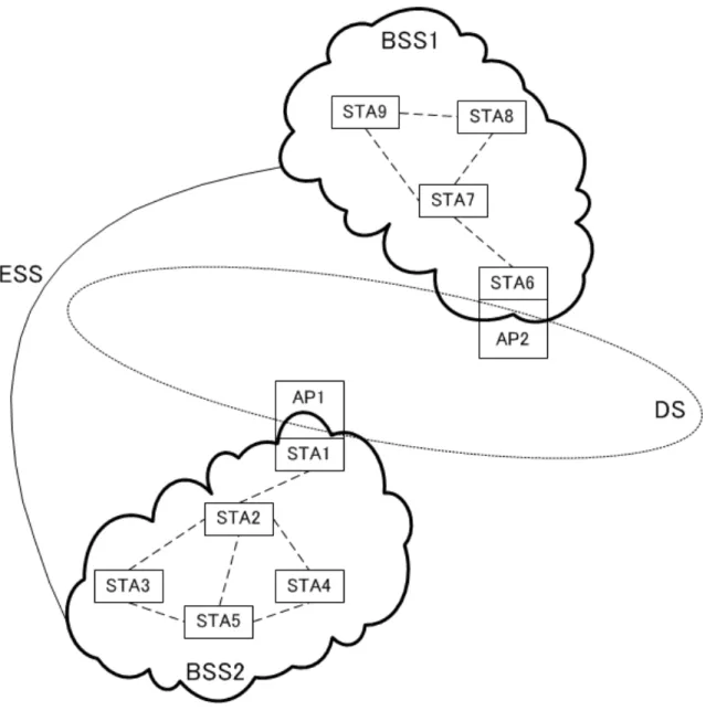
Before introducing the network architecture of WMN, we ﬁrst explain the original IEEE802.11 architecture. The basic service set (BSS) is the basic block of an IEEE802.11 WLAN. Each of BSS has some wireless stations (STAs) as members. The most basic type of IEEE802.11 WLAN is the independent BSS (IBSS). In IBSS, STAs directly com-municate with each other without connecting to access point. This type of network is often referred to as an ad hoc network. An infrastructure BSS also forms a component of IEEE802.11 WLAN. When a STA acts as an access point, it enables access to the distribu-tion system (DS) which handles address to destinadistribu-tion mapping and seamless integradistribu-tion of multiple BSSs. The DS and infrastructure BSSs allows IEEE802.11 to create a wireless network of arbitrary size, which is called an extended service set (ESS) networks. An ESS is the union of the infrastructure BSSs connected by a DS.

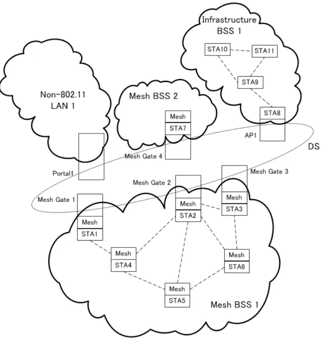
To address the need of wireless mesh in WLANs, a mesh STA is not a member of an IBSS or an infrastructure BSS. Consequently, mesh STAs do not communicate with non-mesh STAs. However instead of existing independently, a mesh BSS (MBSS) also accesses the DS as showed in Fig. 2.1

(13)

Figure 2.1: Example MBSS containing mesh STAs, mesh gates, APs, and portals The MBSS interconnects with other BSSs through the DS. Then, mesh STAs can communicate with non-mesh STAs. A mesh gate works as a router for diﬀerent wireless networks. A portal is a connecter for transmitting frames between 802.11 and non-802.11 LAN. It is possible for one device to oﬀer any combination of the functions of an AP, a portal, and a mesh gate. An example device combining the functions of an AP and a mesh gate is shown in Fig. 2.2. The implementation of such collocated entities is beyond the scope of this standard.

The conﬁguration of a mesh gate that is collocated with an access point allows the utilization of the mesh BSS as a distribution system medium. In this case, two diﬀerent

(14)

entities (mesh STA and access point) exist in the collocated device and the mesh BSS is hidden to STAs that associate to the access point.

Figure 2.2: Example device consisting of mesh STA and AP STA to connect an MBSS and an infrastructure BSS

2.2.1 Features and functions

2.2.2 Hybrid Wireless Mesh Protocol

HWMP is specified in IEEE802.11s Mesh Networking. In HWMP, on-demand routing protocol is adopted for mesh nodes that experience a changing environment, while proac-tive tree-based routing protocol is an efficient choice for mesh nodes in a fixed network

(15)

topology. The demand routing protocol is speciﬁed based on radio-metric ad hoc on-demand distance vector (AODV) routing. The basic features of AODV are adopted, but extensions are made for IEEE802.11s. The proactive tree-based routing is applied when a root node is conﬁgured in the mesh network. With this root, a distance vector tree can be built and maintained for other nodes, which can avoid unnecessary routing overhead for routing path discovery and recovery. It should be noted that the on-demand routing and tree-based routing can run simultaneously.

Four information elements are speciﬁed for HWMP: root announcement (RANN), path request (PREQ), path reply (PREP), and path error (PERR). Except for PERR, all other information elements of HWMP contain three important ﬁelds: destination sequence number (DSN), time-to-live (TTL), and metric.

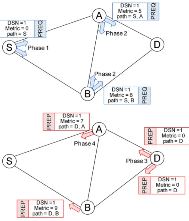
In the HWMP on-demand path selection algorithm (see Fig. 4), a source S wanting to send data to a destination D broadcasts a PREQ frame indicating the MAC address of D. All mesh stations receiving the PREQ create or update their path to S, but only if the PREQ contains a sequence number (denoted as DSN) greater than the current path or the same DSN and a better metric. Every mesh station, before re-broadcasting the PREQ, must update the metric field to reflect the cumulative metric of the path to S. Once D receives the PREQ, it sends S a unicast PREP. If D receives further PREQs with a better metric (and the same or greater sequence number), it sends a new PREP along the updated path. Intermediate mesh stations shall then forward the PREP(s) to S along the best path (stored during the PREQ flooding phase), and, when the PREP reaches S, the path is set up and can be used for a bi-directional exchange of data. If more than one PREP is received, the PREPs following the first are processed only if their information is not stale and announces a better metric (the same rules of PREQ apply). Note that the metric values carried by PREQ and PREP frames refer to two different paths: PREQs measure the reverse path, i.e. from D to S, whereas PREPs measure the forward (S → D) path. This is because the value inserted by each node refers to the metric it measures towards the node from which it received the PREQ/PREP. Hence, depending on the metric computation strategy, it may occur that the forward and reverse paths do not coincide.

(16)

Figure 2.3: Example of the path discovery procedure

2.2.3 Airtime Link Metric

Routing metric is a popular research topic in WMN during recent years. A link metric is a measured unit to a link and a path metric is a value which is assigned to a path, combining by all the link metrics in the path, used by the routing algorithm to select the optimized routes for a speciﬁed objective. The optimization objectives can be minimizing

(17)

delay, minimizing energy consumption, maximizing throughput, etc. The path metric is the combination of the link metrics in the whole path and the method for combining the link metric and the path matric can be deﬁned in varies ways which are depended by the actual situations. The usual functions are summation, multiplication and statistical measures (minimum, maximum, average).

Airtime link metric (ALM) is a default link metric for path selection routing protocol in the IEEE802.11s Mesh Networking. The extensibility framework allows this metric to be overridden by any path metric as specified in the mesh profile. Airtime reflects the amount of channel resources consumed by transmitting the frame over a particular link. This measure is approximate and designed for ease of implementation and interoperability. The airtime for each link is calculated as follows.

Ca= [O + Bt r ] 1 1− ef (2.1) where O and Btare constants, O can be calculated as equation O is equal to the P LCP

preamble length plus the P LCP header length plus the M AC header plus DIF S and

CWmin. The input parameters r and ef are the data rate in bit/seconds and the frame

error rate for the test frame size Bt, respectively. The rate r represents the data rate at

which the mesh STA would transmit a frame of standard size Bt based on current

con-ditions and its estimation is dependent on local implementation of rate adaptation. The frame error rate ef is the probability that when a frame of standard size Bt is transmitted

at the current transmission bit rate r, the frame is corrupted due to transmission error.

2.3 Performance Evaluation

We estimate the frame error rate (FER) as follows. When a packet is sent from one node to another, the power of the signal is attenuated during transmitting. When the packet is received by the target node, we calculate the receiving power by the two-ray fading model:

PRX = PT X· G (2.2)

where the G is deﬁned as (2.3) for which the unit of input power and output power is Watt.

G = 1

d4 (2.3)

The signal-to-noise rate (S/N) can be estimated as (2.4).

SN R = PRX

PAW GN

(2.4) We convert the unit of AWGN from mW to dBm using (2.5).

PdBm= 10log10

PmW

(18)

And we get the AWGN as following.

PAW GN = 10

−108dBm

10 = 1.58× 10−11mW (2.6)

According to Zhi Ren’s result, the average bit error (BER) for QAM64 with Rayleigh fading is as (2.8) after we change the S/N to logarithmic decibel scale using (2.7).

SN RdB = 10log10SN R (2.7)

BER≈ 7

6× 10SN RdB/10 , if BER > 1, we set : BER = 1. (2.8)

Then we obtain the average BER and the FER equation as (2.9) and (2.10).

BER≈ 1.85× 10 −11 PT X· d−4 (2.9) F ER = BER× 8192 = 1.51× 10 −7 PT X · d−4 (2.10) The constants used for these equations are listed in the following table.

Parameter

Value

P LCP preamble length 20µs

P LCP header length

4µs

M AC header

69.33µs

DIF S

34µs

CW

min

135µs

B

t

8192bits

P T X

54M bps

P

dBm

100mW

r

−108dBm

2.3.1 ALM performance

In order to analyze the performance of ALM, the airtime cost metric versus distance is simulated and showed in Fig. 2.4. According to the Figure, when the distance is less than 30 meters, the ALM value is nearly constant, which are around 410µs. Then, it increases exponentially for the following distance. The result indications that airtime link metric is not practical for short distance cases. Based on theoretical study, IEEE 802.11a is usually implemented in transmission range over 250 meters with the rate of 54Mbps. However, our simulation transmission range is around 100 meters; therefore this airtime link metric formulate is not suitable to use for indicate the nearest MPP for our condition.

(19)

We modify the existing airtime link metric formulate so that the airtime link metric can provide a clear diﬀerence between each distance interval.

Figure 2.4: Airtime link metric versus distance

We have made some modiﬁcation to the original ALM, and called this new ALM as

CaEx.

CaEx = Ca· (1 +

d dR

) (2.11)

where Ca is the original ALM, d is distance and dR is transmission range. The modiﬁed

ALM now is depend on the transmission range for speciﬁc coverage area of WMN envi-ronment. Fig. 2.5 shows the comparison between the original ALM (Ca) and the new

ALM (CaEx). The ALM values of CaEx are increased dramatically with the increased of

distance. It is obvious that the values of CaEx have a larger variance for each distance

in-terval compare to ALM of Cawhich provide nearly the same results for the ﬁrst 50 meters.

(20)

Figure 2.5: Modiﬁed/Unmodiﬁed ALM versus distance

2.3.2 Single MPP

In this section, we study the performance of the ALM over the HWMP protocol in the WMN environment. We use C++ console application to construct and simulate the WMN environment. This program is event-driven application. All the events are defined in the configuration file. In the program, we simulate each mesh station as a independent object. Each mesh station has its own properties. In the startup, the application first reads the configuration file to initialize the parameters and generate all the events. When an event meets its time, it will be forwarded to the specified node to process event.

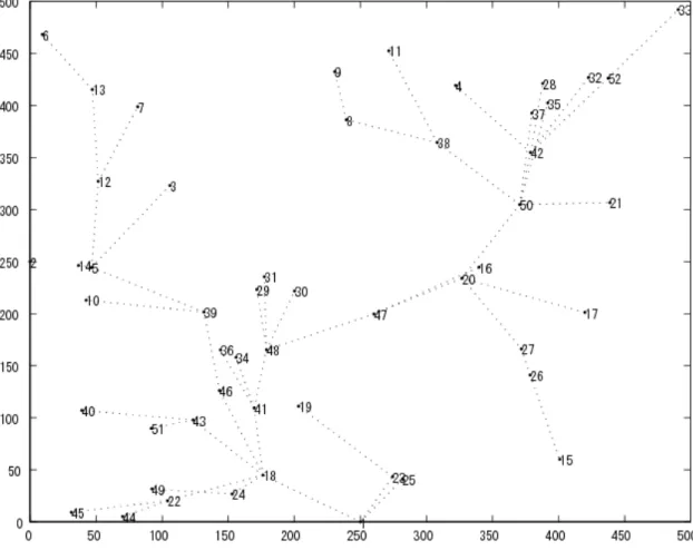
In our simulation, all the mesh stations that included two MPPs are confined to a 500m× 500m area. One MPP is located at (250, 0) and another one is located at (0, 250) whereas other mesh stations are placed randomly and distributed. Other parameters are summarized in Table 1. We model our traffic based on constant bit rate (CBR). All source mesh stations are chosen to send their data to the MPP. The CBR traffic consists of 1000-byte frame size, which sends at the constant data sending interval.

(21)

(22)

Figure 2.7: Tree topology for MPP at (0, 250)

2.3.3 Nearest MPP (NMPP) Solution

In the existing research work, the Nearest Gateway (NGW) solution is used to assign each MAP or MP to its nearest gateway through routing metric hop count. However, ALM is used in our study to allocate each MAP or MP to connect with the serving MPP with routing metric. We define this technique as Nearest MPP (NMPP) solution. NMPP chooses the flow in between source and destination with the smallest ALM value from single MPP data traffic results for data transmissions. Fig. 2.8 shows the tree topology that generated by NMPP solution. It is clear that the amount traffic flows for different MPPs are generated without any optimization algorithm. Therefore, we proposed a novel load balance optimization algorithm in chapter 3 to resolve the problem in NMPP solution.

(23)

Figure 2.8: Tree topologies using NMPP solution

2.4 Simulation Results and Discussion

In order to understand the characteristics and performance of single MPP and NMPP solution, we have constructed the simulation to investigate the latency in second with number of node and the latency in second with the data sending time interval. The results of the simulations are shown in Fig, 2.9 and Fig. 2.10 respectively. The latency in this context means the average elapsed time to deliver a packet from the source to the destination, which includes all possible delays before data packets arrive at their destinations, e.g. queue time, propagation delay, and others.

In Fig. 2.9, the latency is increased proportionally with the number of nodes. The NMPP, single MPP at (250,0), and single MPP (0,250) have nearly same increment pattern. The single MPP at (250,0) and single MPP (0,250) have the same latency value, 0.082 and 0.09 when the number of nodes is 30 and 40 respectively. The latency of NMPP is 22.5% lower than both single MPP at (250,0) and (0,250). Therefore, we can say that the NMPP is performed better than single MPP. This is due to the tracs around the single MPP of the tree- topology becomes signicantly less when the NMPP is forced to share

(24)

the trac load with other MPP. This leads to the fact that the number of packet drops due to packet collision and buer overow reduces largely as well as a decrement of packet processing and forwarding at the NMPP.

For the latency versus data sending interval as showed in Fig. 2.10, when the data sending interval is increased, the maximum latency of NMPP, single MPP at (250,0) and single MPP at (0,250) is decreased. The latency of NMPP is 20.8% lesser than both single MPP at the data sending interval 0.1 seconds. The results of latency for single MPP at (250,0) and single MPP (0,250) is almost the same for the variance data sending interval. The latency of both single MPP is getting closer to latency of the NMPP when the data sending interval is increased. The latency for single MPP is approximately same with latency of NMPP, which is 0.10 seconds at the data sending interval of 10 seconds. The NMPP can achieve better performance than single MPP when the data sending interval is smaller, because the NMPP consists of smaller airtime cost in routing the data messages with the best-metric route that shared with other MPP. As the result, the average latencies by applying the NMPP solution between the source and destination are lower than the cases of the single MPP.

(25)

(26)

Chapter 3 Traﬃc Balancing Algorithm for

Multiple Portal

3.1 Introduction

In this chapter, we address the traffic balancing problem in WMNs by proposing a novel algorithm, called optimal latency balancing with depth-first search (OLB-DFS) algorithm, which enables to perform traffic balancing among the multiple mesh gateways. Our aim is to propose and evaluate the proposed OLB-DFS algorithm over the HWMP protocol in the WMNs environment with multiple mesh gateways. Our contribution is divided into three folds. First, we model the traffic balancing problem based on the latency metric and define this problem can be optimized by our proposed OLB-DFS algorithm. Second, we use the depth-first search (DFS) method to fasten the domain weight computation at the mesh gateway with a low memory. Third, this research shows the investigation of the performance of the OLB-DFS algorithm under the multiple mesh gateway WMNs environment. Our proposed OLB-DFS algorithm executes periodically and adapts to the dynamic network change. It can use to balance the traffic load among the MPPs and improve the latency of packet sending. It also effectively can find the potential traffic flows to be switchable until the inter-domain traffic volume is balanced. As a result of applying the OLB-DFS algorithm, latency, network throughput and packet delivery ratio are improved.

3.2 Preliminaries

3.2.1 Network Model and Assumptions

A MAP is a MP that works as an access point to receive or send the Internet traﬃc for the associated MSs. For the sake of simplicity, the abbreviations MAP and MP refer to the ‘MAP’ and are indistinguishably interchangeable. Let N be the set of MAPs of a WMN, we assume that MAPs, n ={1, 2, . . . , N } ∈ N are distributed in a two-dimensional plane and have equal communication range. The network topology is modeled as a connected

(27)

graph, G(N , E). An edge {u, v} ∈ E iff. the distance between MAPs u and v is within each other’s communication range. The latency between two adjacent MAPs u and v can be defined as λ(u, v). We assume that λ(u, v) = λ(v, u). The minimum latency between any source-destination in the network is the λ-cost of the shortest path connecting them that defined with the ALM function. The Dijkstra algorithm can be utilized to construct a shortest path rooted by the source. Routes inside the WMN are given by the HWMP routing protocol. Since a MS is logically and wirelessly connected to a MAP, a user through the MS initiates connections to the Internet, which can generate downlink flows or uplink flows in between MAP and MPP. Let G be the set of MPPs in the WMN. Let

F be the set of downlink or uplink flows. A flow can be routed through different paths

from each MAP to the MPP and vice versa. Let f ={1, 2, . . . , F} ∈ F is the set of active ﬂows. Let Dg be the set of domains that containing the set of active ﬂows served by the

set of MPPs, g ={1, 2, . . . , G} ∈ G. Each domain D can generate a domain weight, called

W. Let Wg be the set of domain weights that containing the sum of the path routing

weights for each source-destination paths of the corresponding domainDg. Therefore, the

domain weight can be written as

Wg = fg

∑

i∈F;i=1

wi (3.1)

This path routing weight (wi) is decided by using the routing metric, i.e., hop count,

delay, bandwidth, energy per bit, airtime cost, etc. In our research, the path routing weight is decided by the latency parameter. Thus, the path routing weight of the ith ﬂow can be expressed as

wi = λi(S, D) (3.2)

where S denotes source and D denotes destination. If we consider two MPPs and fifty MAPs in a WMN, then g is equal to 2 and n is equal to 50. If all the MAPs have a flow to the MPPs, then f is equal to 50 flows. The routing protocol will divide all the flows into two domains served by two MPPs, respectively. This also means thatD1 and D2 contain

W1 and W2, respectively.

3.2.2 Problem Statement

Internet traffic directed to a MAP will be served by MPPs; the traffic is routed from the MPP to the MAP using a minimum cost path (in terms of the routing metric used) and vice versa. The MPP load-balancing problem requires choosing the serving MPP function for every downlink or uplink flow. The problem concerns Internet traffic at the MPP, because it accounts for most of the network load. One of the alternative solutions for the HWMP protocol to deal with multiple portal is the Nearest MPP (NMPP) solution, which assigns each MAP to its nearest MPP in terms of the ALM routing metric. The NMPP solution can easily lead to load imbalance (e.g. Fig. 3.1) because of the local decision of selecting link through metric without any optimization algorithm. To deal with this problem, we first formulate that P is the traffic balancing problem for multiple

(28)

portal in a WMN. P is also an optimization problem. A solution of P must choose the serving MPPs can be balanced with the most minimum value of C variable. Let

C = min{diﬀ (W1,W2, . . . ,WG} be the achievable value in a WMN. Given the above

considerations, the problem can be formulated as:

P : minimize diﬀ (W1,W2, . . . ,WG) (3.3)

subject to C ≥ 0 (3.4)

TheP is NP-hard so any deterministic algorithm can not solve the problem in polynomial time. So, exact algorithm for solving this problem can be only used for small scale instances because the execution time of such kind of algorithms exponentially increases with the problem dimensions. For larger instances (containing hundreds or thousands of vertices), the only way to achieve quality results is to use some heuristic methods. The next section describes our proposed solution for solving this problem.

(29)

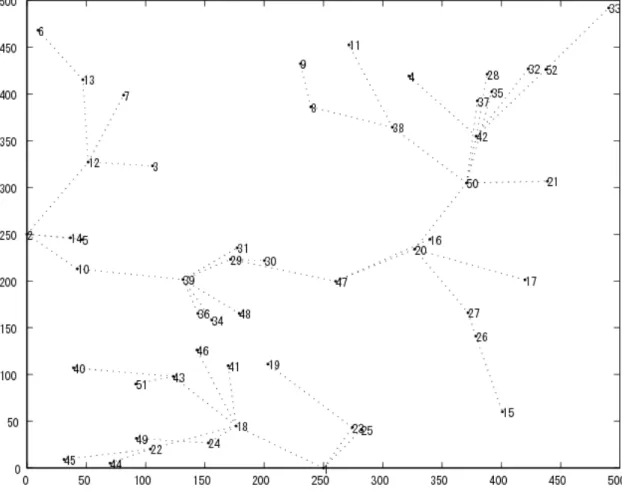
Figure 3.2: Network topology that generated by the OLB algorithm

3.3 Optimal Latency Balancing Algorithm

Most of the cases, WMN is not used independently. WMN is designed to access to other types of wired networks. For such purpose, the function of MPP that acts as root node is very essential. In our research, we focus on proposing a feasible path metric for the HWMP and a traffic balancing algorithm for the multiple portal in WMN. Since the ALM that specified in IEEE802.11s reflects the amount of channel resources consumed by transmitting the frame over a particular link. This measure should be transformed in a generic path metric, i.e., latency. In our research, latency for a wireless network is defined as the time of the start of packet transmission at the source node to the time of the end of packet reception at the destination node. This latency does not comprise of the time to process the packet at both source and destination nodes. It is important to distinguish between network latency and latency to avoid confusion. Since the network latency can be measured either one-way (the time from the source sending a packet to the receiving destination) or round-trip (the sum of the one-way latency from source to destination and the one-way latency from destination to source), we interpret latency metric is similar to the one-way network latency.

(30)

3.3.1 Proposed Solution

We propose an optimal latency balancing with depth-first search (OLB-DFS) algo-rithm, dynamically computes the domain weight of MPPs and balances the traffic that are directed to/from a wired network through the serving MPP. Because users are ran-domly accessed to the MAP and can generate connections at any time, network conditions can constantly change. It is therefore important that the algorithm adapt to the current conditions, and the solution must converge, while avoiding route flapping. The proposed OLB-DFS algorithm is an adaptive algorithm, which continually monitors the network conditions of WMN. Based on the current conditions and the knowledge of the network topology, the proposed OLB-DFS calculates a solution P. The OLB-DFS algorithm is self-corrective and executes periodically to adapt to current conditions. The basic idea of the OLB-DPS algorithm is to balance the traffic load among the MPPs in order to increase inter-domain flow fairness and minimize the latency of packet sending.

Through the HWMP protocol with the ALM criterion, the traﬃc of the MAPs can be transfered to the serving MPPs with the shortest path. The OLB-DFS algorithm starts with the path routing weight computation for each active ﬂows of the WMN. Then, the OLB-DFS algorithm the initial solution of P = Cinitial. To guarantee an optimal

solution ofP, it is impossible to evaluate every possible solution due to time and memory limitations. Therefore, a DFS method is used to ﬁnd the feasible solution quickly so that the algorithm can compare the feasible solution with initial solution. During the iteration process, the DFS method looks for possible feasible solution and increase the balance of the domain weights by ﬁnding the optimal solution of P = Coptimal.

The general idea of DFS method is as follow. Each MAP memorizes if it has already been visited by the DFS traversal, and the sender from where the traffic flow was re-ceived for the first time. The MAP that is currently holding the routing table will sort all its unvisited neighbors by the ALM criterion. The first MAP in the list of routing table is selected to transport the traffic flow. If a MAP has no unvisited neighbors to proceed, it returns to itself as the sender, which will transport the traffic flow to the next

unvisited neighbor in the list of routing table. Eventually, the traﬃc ﬂow either reaches

the destination, or returns back to the source, which has no unvisited neighbors. The OLB-DFS algorithm that integrates latency criterion with DFS operates as presented in

Algorithm 1. Table I lists the symbols used to explain the OLB-DFS algorithm. The

OLB-DFS algorithm executes every ﬁxed period of time, which should be greater than a few times of PREQ broadcast interval time. To improve the inter-domain ﬂow fairness, the OLB-DFS algorithm will attempt to switch MPPs from domains D1 with an above

average number of ﬂows to domains D2 with a below average number of ﬂows. If

switch-ing from D1 to D2 is not suspended, the OLB-DFS algorithm progressively ﬁnds other

flows to be switchable until the optimal solution of P is achieved. To avoid the same flow switch back to the original domain, the OLB algorithm can use the ‘scavenge stale resource record’ to prevent oscillations. The topology generated by OLB algorithm can be seen in Fig. 3.2. Comparing with Fig. 3.1, we can see that the flows to each MPP are balanced by the OLB algorithm. Through balancing the weight of each domain, the OLB algorithm have potentially improved the network latency and throughput that we

(31)

will described in the next chapter.

Table 3.1: List of Symbols

Symbol

Description

G

Set of MPPs

D

Set of domains

F

Set of downlink or uplink ﬂows

(32)

Algorithm 1 Optimal Latency Balancing with Depth-ﬁrst Search (OLB-DFS)

01: Deﬁnition: S is source, D is destination.

02: Input: all the pairs of S and D, the path routing weight wSD.

03: Output: an optimum value of C with the switch ﬂows. 04: Begin

05: C = 0; // C is a variable of optimization value.

06: Set g =G parameter // g is the number of serving MPPs in a WMN. 07: Compute Wg and C;

08: C = C;

09: Set Wmax = max{Wg};

10: Set Wmin = min{Wg};

11: Set wSD = argmax{Wmax}; // Set the highest path routing weight.

12: Choose S from wSD;

13: S is marked as visited ; disconnected ﬂag = 0;

14: for Dmin do {

15: A = S; // A is the next MAP.

16: while D is not reached && disconnected ﬂag = 0 do {

17: if A = S // S has no unvisited neighbors

18: disconnected ﬂag = 1; // S and D are disconnected

19: if A ̸= S && A has no unvisited neighbors

20: return to itself; A = sender to A; 21: if A has unvisited neighbors

22: A sorts all unvisited neighbors using ALM criterion;

23: A sends the packet to the ﬁrst neighbor B in the list;

24: B memorizes A as the sender ;

25: B is marked as visited ;

26: A = B;

27: } 28: }

29: if disconnected ﬂag = 1

30: Go to the line 11 with the next highest path routing weight; 31: else

32: Switch the ﬂow of S to the Dmin domain;

33: Compute Wg and C

′

; 34: if C′ ≥ C

35: C = C′;

36: Go to the line 9 for the next domain weight; 37: else

38: Break; 39: End

(33)

3.3.2 How the Proposed Protocol and OLB Algorithm Work

In our proposed routing protocol, we use HWMP as base protocol. We choose proac-tive mode of operation in the HWMP. We can generate tree topology network for each MPP respectively by issuing root announcement (RANN) from specified MPP with the ALM metric. By this method, each MAP/MP can create a routing table for each MPP separately. Through the different routing table MAP/MP can send data packet to the different destination MPP. When all the MAP/MP choose the path with the same des-tination, it is a single MPP transmission. If all the MAP/MP choose the path with the best ALM metric value, it is the NMPP solution for multiple portal. For our proposed algorithm, we use the latency as another metric. We get sets of uplink latency metrics to each MPP through a period time of data transmission of each single MPP traffic. The latency value is inside the payload of data packet. The MPPs will calculate the average latency for each flow and share their average latencies. One of the MPP will perform OLB algorithm to partition the topologies. The MPP will send the extended PREQ mes-sage with the latency metric and next hop address and MPP address to each MAP/MP. When MAP/MP receives PREQ message, it will update its routing table and send PREP through the new path to the destination MPP. For the case of downlink, the MPPs send PREQ messages to each MAP/AP after a period time of data traffic. When MAP/MP receives PREQ message, it will first calculate the average latency from this MPP and reply the PREP message with this average information. Through the information which are get from MAPs/MPs, one of the MPP will perform OLB algorithm and send the routing table contents to each MAP/MP by PREQ message. When MAP/MP receives this kind of PREQ message, it will update its routing table and send back PREQ message to the specified MPP.

For the MAP/MP states and traffic conditions usually change, the RANN message will send again periodically. Inside the interval time the RANN message send, the MPP is configured that it will also periodically process the traffic balancing algorithm. E.g. the PREQ message for sending routing table contents and collecting latency for OLB algo-rithm will be issued periodically. The interval of processing OLB algoalgo-rithm is less than that of sending RANN message. By this way, the protocol always behaves smart and adaptively. Therefore, the traffic load in the network is always optimal balanced.

3.4 Performance Evaluation

We evaluate and study the performance of the proposed OLB-DFS algorithm over the HWMP protocol in the WMN environment with multiple portals and a varying number of flows. We use C++ console application to construct our simulator program. This program is event-driven application. All the events are defined in the configuration file. In the program, we simulate each MAP as a independent object. Each MAP has its own properties. In the startup, the application first reads the configuration file to initialize the parameters and generate all the events. When an event meets its time, the gener-ated packets will be forwarded to the specified MAP to process event. We compare our

(34)

proposed OLB-DFS algorithm with the NMPP solution.

3.4.1 Simulation Environment and Setup

The IEEE802.11a hardware speciﬁcation with CSMA/CA protocol is used to investi-gate the performance of proposed OLB-DFS algorithm and the NMPP solution over the HWMP protocol in the WMN environment. The parameter types and values are shown in Table II. In our simulation, two serving MPPs are considered as a preliminary stage of performance evaluation studies. One MPP is located at (250 m, 0) and another one is located at (0, 250 m) whereas other MAPs are randomly distributed over 500 m× 500 m ﬁeld. We assume that all the MAPs are identical. This means MAPs have same transmit power and transmission bit rate. We assume that all the MAPs is static throughout the entire simulation.

We model our traffic based on user datagram protocol (UDP). MAPs connect to the serving MPP, which generates downlink and uplink flows. For each MAPs, the time between start of connections follow an exponential distribution with ten seconds. The UDP traffic consists of 1000-byte frame size, which sends at the exponential distribution with traffic interval of one second. We ran our simulation for 10 minutes and 10 topologies with different seeds for pseudo-random number generator are averaged. In our simulations, we focus the influence of the number of flows and number of nodes on the performance of the OLB-DFS algorithm and the NMPP solution over the HWMP protocol. To observe the effect of flow increment, we vary number of flows from 10 to 50 flows in increment of 10 flows for both uplink and downlink flows. To evaluate the performance of node increment, we change number of nodes from 10 to 50 in increment of 10 nodes and fix the number of flows to 10 flows for both uplink and downlink traffics.

(35)

Table 3.2: Simulation parameters and settings

Hardware speciﬁcation

IEEE 802.11a

MAC protocol

CSMA/CA

Maximum contention window 1023

Minimum contention window

15 PLCP preamble length

20 µs

PLCP header length

4 µs

Slot time

9 µs

SIFS

16 µs

DIFS

34 µs

Network protocol

HWMP

PREQ size

28 bytes

PREP size

24 bytes

PREQ interval

15 s

Number of MPPs

2 Network coverage

500 m

× 500 m

Energy model

Two-ray

Propagation loss exponent

4 Transmit power

100 mW

Pattern of MAP

static

Transmission bit rate

54 Mbps

Queue size

100 packets

Traﬃc type

UDP

Traﬃc interval

100 ms

Data payload size

1000 bytes

Data header size

24 bytes

3.4.2 Performance Metrics

The simulation results are observed with four sets of performance metrics; latency, network throughput, hop count, and packet delivery ratio. Latency is the average end-to-end delay of all delivered data packets of all the ﬂows. Hop count is the average end-to-end-to-end-to-end hop count of all the source and destination pairs. Network throughput is the total data bytes delivered by the network divided by the time elapsed since the ﬁrst packet was sent and the last packet was received. Packet delivery ratio is the ratio of received data packets to those transmitted by the source.

(36)

Figure 3.3: Latency as a function of number of ﬂows. Table 3.3: Hop count as a function of number of ﬂows

Number of ﬂows

10

20

30

40

50 Uplink

NMPP

4.17 4.10 3.94 3.87 3.78

OLB-DFS 4.48 4.43 4.36 4.26 4.18

Downlink

NMPP

4.45 4.36 4.31 4.21 4.10

OLB-DFS 4.63 4.50 4.45 4.39 4.37

(37)

(38)

Figure 3.5: Packet delivery ratio as a function of number of ﬂows.

3.4.3 Simulation Results and Discussion

3.4.3.1 Part 1: Performance eﬀect on varying the number of ﬂows

It is essential to note that each value shown in the graph is the average value taken from ten different topologies. Fig. 3.3 shows the performance for the latency versus the number of flows. We can obtain that OLB-DFS outperforms NMPP significantly as number of flows increases. The reason for this behavior is the possibility of switching flow is getting increase as number of flows increases. OLB-DFS can decrease the latency by average of 16.1% and 4.5% for the uplink traffic and downlink traffic, respectively. For the uplink traffic, when the traffic is very crowed (i.e., 50 flows), OLB-DFS outperforms NMPP 30.8%. This means when the load traffic is full, the OLB-DFS algorithm will perform a maximum improvement for the traffic balancing of multiple MPPs. When the number of flows is 10 and 20, we can see that the OLB-DFS algorithm and NMPP solution almostly perform the same. The reason for this is that when the network traffic is low, the latency is small so that the with the NMPP solution usually performs well and the network condition does not need to be balanced. In this case, the OLB-DFS algorithm makes less effect. Also for the downlink traffic, the network traffic is not crowed enough to make congestions. The data senders are only the two MPPs. In this condition, the OLB-DFS algorithm does not outperform NMPP obviously.

(39)

From Table III, we can observe this phenomena that by using OLB-DFS algorithm, the average hop count increases while comparing with applying NMPP solution.

Fig. 3.4 shows the performance for the network throughput versus the number of flows. With a small number of flows there is no contention and so the improvement achieved by OLB-DFS is small. As the number of flows goes up, the throughput of flows de-creases for NMPP but by OLB-DFS is able to improve flow throughput and therefore the network throughput is increased. OLB-DFS is noticeably achieved network throughput improvement for the uplink traffic and the downlink traffic are about 8.7% and 12.2%, respectively. When the number of flows is larger than 20, the entire network throughput for the uplink traffic is higher than the downlink traffic. This is because when the flow increase, the number of uplink packets of the whole network increases faster than that of the downlink traffic.

As the number of flows increases, contention in the network increases, which leads to packet drops. The performance for packet delivery ratio is shown in Fig. 3.5. For the up-link traffic, generally NMPP drops faster. OLB-DFS performs slightly better than NMPP. The packet delivery ratio drops slightly with OLB-DFS, which indicates that it can effec-tively balance the entire inter-domain traffic fairness. From different viewpoint, we can see that the traffic becomes imbalance when the number of flows increases. This leads to the packet delivery ratio decreases. This reason is that increasing traffic imbalance progressively produces high contention and more interference in one domains. However, OLB-DFS is less affected by this issue, because it can self-corrective and dynamic mon-itoring the traffic always in the balance mode. For the downlink traffic, because of the low traffic load, the OLB-DFS and NMPP are both with no packet loss.

(40)

Figure 3.6: Latency as a function of number of nodes. Table 3.4: Hop count as a function of number of nodes

Number of nodes

10

20

30

40

50 Uplink

NMPP

1.95 2.75 3.07 3.89 4.37

OLB-DFS 1.97 2.70 3.22 3.88 4.48

Downlink

NMPP

1.94 2.58 3.23 3.92 4.45

OLB-DFS 1.99 2.60 3.21 4.00 4.33

(41)

(42)

Figure 3.8: Packet delivery ratio as a function of number of nodes.

3.4.3.2 Part 2: Performance eﬀect on varying the number of nodes

In this part, the performance results are obtained by fixing the number of flows is 10 for both uplink and downlink flows. Fig. 3.5 shows the performance for the latency versus the number of nodes. When the number of nodes increases, the latency is also increased. The downlink and uplink traffic performs almost the same for both NMPP and OLB-DFS algorithm. One of the reason is when the number of flow is 10, the traffic load of the whole network is low so that with the NMPP solution, the average latency is already very low, and OLB-DFS cannot easily make any improvement here. Another reason is that the implementation of the OLB-DFS algorithm is not well tested. For the OLB-DFS algorithm should have improvement here for the minimization of the latency of the whole network and the balancing of the multiple MPPs.

Table IV shows that the average hop count versus number of nodes. The average hop counts are almost the same for both OLB-DFS algorithm and NMPP solution.

Fig. 3.6 shows the performance for the network throughput versus the number of nodes. When the number of nodes increases, the network throughput also increases. We can see that with a small number of nodes the traffics are very low, the network throughput are also very low for both uplink and downlink traffics. When the number of nodes is larger than 20, the throughput of the downlink traffic is larger than that of the uplink traffic. In this case, the OLB-DFS almost achieved no improvement comparing with NMPP.

(43)

The performance for packet delivery ratio is shown in Fig. 3.7. As the number of nodes increases, the packet loss is alway 0 for both OLB-DFS algorithm and NMPP solution.

3.5 Concluding Remarks

In our research, we addressed the advantages of multiple portal for attaining the high traffic volume that goes through single mesh gateway. We therefore proposed the OLB-DFS algorithm for the HWMP protocol to be able to handle the issue of multiple portal in the WMN environment. The key features of the OLB-DFS algorithm are as follow. (i) it can use to balance the traffic load among the MPPs; (ii) it can use to improve the latency of packet sending; and (iii) it effectively can find the potential traffic flows to be switchable until the inter-domain traffic volume is balanced.

We also examined the performance of the OLB-DFS algorithm compared to the NMPP solution over the HWMP protocol under the multiple portal WMN environment. Simula-tion results reveal that the OLB-DFS algorithm can attain a high reducSimula-tion of latency by up to about 30.8% for the uplink traffic and also can accomplish an improvement in the network throughput by up to about 8.7% for the uplink traffic. In addition to that, the OLB-DFS algorithm can achieve a merely improvement in terms of packet delivery ratio. For this evaluation it can be concluded that using the OLB-DFS algorithm can provide good advantages and beneficial to the routing protocol for the WMN environment.

(44)

Chapter 4 Conclusion and Future Work

4.1 Concluding Remarks

In our research, we have studied ALM which is a default link metric of WMNs, and we found the restriction of ALM that it performs weak in short distance wireless transmission. We proposed a modified outperformed ALM placing with the original ALM and based on the modified ALM to do rest of our research. We simulated the scenarios to exam the performance of WMN with single MPP. We also evaluate the cases with wireless mesh networking with multiple MPP by selecting the link with the best metric value. The result that the average latency for the whole network is dramatically reduced but the method did not consider the traffic balancing for the multiple portal’s problem, that part of MPP might be quite crowed so that it causes high latency and high packet loss rate.

Considering with the traffic load balancing problem, we proposed a load balancing algorithm named OLB-DFS. We simulate the algorithm in our WMN simulator. We also model our traffic into two different types: downlink flow and uplink flow. We evaluated our algorithm through the two different types, and we get a result of about 16.1% improvement comparing with the NMPP solution for the uplink traffic. The multiple portal issue was reduced that the latency of the whole WMN was reduced and the multiple portal’s load balancing problem was also reduced.

4.2 Research Contributions

There are three contributions in our research.

(1) We have written a general simulator to simulate the WMN environment. By using the simulator, we evaluate the performance of ALM and proposed a modiﬁed version of ALM for the unpractical reason in the case of low distance.

(2) We have evaluated NMPP solution and compare the results with single MPP routing in terms of number of nodes and data sending interval.

(45)

(3) We have proposed OLB-DFS algorithm to balance the traﬃc load for the multiple portal in WMN, and we get a good result that the network obtained average low latency, high network throughput, and low packet loss rate than the NMPP solution in uplink traﬃcs.

4.3 Future Works

(a) For the OLB algorithm performs not well when traffic is downlink and the number of flows is less than 20, we will try to find reason in the implementation of OLB algorithm and we also will make more simulation topologies to simulate the problem and try to get good results.

(b) In future, the interference in the topologies will be considered into OLB algorithm to reduce unstable results on packet loss rate and latency.

(c) In WMNs, the data traﬃcs are usually TCP. So, we should evaluate the OLB algorithm in TCP traﬃc.

(d) We will examine the OLB algorithm when the number of MPPs is larger than 2. (e) Our evaluations of OLB algorithm are focused on the ﬁxed topology in the WMNs.

We will also investigate the performance of OLB in the WMN environment with the mobility issue.

(f) The placement of MPPs will be investigate to improve the performance and traﬃc load balancing in WMNs.

(46)

References

[1] F. Akyildiz et al., “Wireless mesh networks: a survey,” in Elsevier Computer

Net-works Journal, vol. 47, no. 4, pp. 445―487, Nov. 2005.

[2] K. W. Lim et al., “Congestion-aware Multi-Gateway Routing for Wireless Mesh Video Surveillance Networks,” in Sensor, Mesh and Ad Hoc Communications and

Networks (SECON), 2011 8th Annual IEEE Communications Society Conference,

Salt Lake City, Utah, USA, Jun. 2011, pp. 152-154.

[3] S. Maurina et al., “On tree-based routing in multi-gateway association based Wireless Mesh Networks,” in Personal, Indoor and Mobile Radio Communications, 2009 IEEE

20th International Symposium, Tokyo, Japan, Sep. 2009, pp. 1542-1546.

[4] J. J. G´alvez et al., “A Feedback-based Adaptive Online Algorithm for Multi-Gateway

Load-Balancing in Wireless Mesh Networks,” in World of Wireless Mobile and

Multi-media Networks (WoWMoM), 2010 IEEE International Symposium, Montreal,

Que-bac, Canada, Jun. 2010, pp. 1-9.

[5] IEEE Computer Society, IEEE Std. 802.11s-2011: Standard for Local and

metropoli-tan area networks, Part 11: Wireless LAN Medium Access Control (MAC) and Phys-ical Layer (PHY) speciﬁcations, Amendment 10: Mesh Networking IEEE Computer

Society Std., Sep. 2011.

[6] Z. Ren et al., “Modeling and simulation of fading, pathloss, and shadowing in wireless networks,” in Communications Technology and Applications, 2009. ICCTA’09. IEEE

International Conference, Beijing, China, Oct. 2009, pp. 335-343.

[7] I. Akyildiz, and X. Wang, Wireless mesh networks. Vol. 3 Wiley, 2009.

[8] S. Methley, Essentials of wireless mesh networking Cambridge University Press, 2009. [9] B. H. Walke et al., IEEE 802 wireless systems: protocols, multi-hop mesh/relaying,

performance and spectrum coexistence Wiley, 2007.

[10] Y. Zhang, Wireless mesh networking: architectures, protocols and standards Auer-bach Pub., 2007.

(47)

[11] A. O. Lim et al., “A hybrid centralized routing protocol for 802.11s WMNs,” in

Mobile Networks and Applications (MONET), Monterrey, Mexico, Nov. 2008, vol.

13, no. 1-2, pp. 117-131.

[12] D. Matic, and B. Milan, “Maximally balanced connected partition problem, graphs application and education,” in The teaching of mathematics Sterling Publishers Pvt. Ltd., 2012, vol. 15, no. 2, pp. 121-132.

[13] T. Mutter, “Partition-based network load balanced routing in large scale multi-sink wireless Sensor Networks,” M.S. thesis, Dept. Elect. Eng., Math. and Comp. Sci., Enschede, Netherlands, University of Twente, 2009.

[14] X. Wang and A. O. Lim, “IEEE 802.11s wireless mesh networks: Framework and challenges,” in Ad Hoc Networks Elsevier, Aug. 2008, vol. 6, no. 6, pp. 970―984. [15] R. G. Garroppo et al., “A joint experimental and simulation study of the IEEE

802.11s HWMP protocol and airtime link metric,” in Int. J. of Commun. Syst vol. 25, pp. 92―110, 2012.

[16] J. Guerin et al., “Routing metrics for multi-radio wireless mesh networks,” in

Telecommunication Networks and Applications Conference (ATNAC), 2007 Aus-tralasian Christchurch, New Zealand, Dec. 2007, pp. 343―348.

[17] U. Ashraf et al., “Route selection in IEEE 802.11 wireless mesh networks,” in

Telecommunication Systems Springer, 2011, pp. 1-19.

[18] S. H. Lee and Y. B. Ko, “An eﬃcient multi-hop ARP scheme for wireless LAN based mesh networks,” in Operator-Assisted (Wireless Mesh) Community Networks, 2006

1st Workshop IEEE, Berlin, Germany, Sept. 2006, pp. 1-6.

[19] Y. Kim et al., “Load-balanced mesh portal selection in wireless mesh network,” in

Military Communications Conference, 2007. MILCOM 2007 IEEE, Orlando, Florida,

USA, Oct. 2007, pp. 1-6.

[20] Campista M. E. M. et al., “Routing metrics and protocols for wireless mesh networks. Network,” in Network IEEE 22.1 (2008): 6-12.

[21] A. Kumar et al., “Multicasting in wireless mesh networks: Challenges and opportuni-ties,” in Information Management and Engineering, 2009. ICIME’09. International

Conference IEEE, Kuala Lumpur, Malaysia, April 2009, pp. 514-518.

[22] Y. Yang et al., “Designing routing metrics for mesh networks,” in IEEE Workshop

on Wireless Mesh Networks (WiMesh) IEEE, Santa Clara, CA., Sept. 2005.

[23] P. Georgios et al., “Routing metrics for wireless mesh networks,” in Guide to Wireless

(48)

[24] K. Yang et al., “Hybrid Routing Protocol for Wireless Mesh Network,” in

Compu-tational Intelligence and Security, 2009. CIS ’09. International Conference IEEE,

Beijing, China, Dec. 2009, vol. 1, pp. 547-551.

[25] Nandiraju N.S. et al., “Multipath Routing in Wireless Mesh Networks,” in Mobile

Adhoc and Sensor Systems (MASS), 2006 IEEE International Conference IEEE,

Vancouver, BC, Canada, Oct. 2006, pp.741-746.

[26] D. Richard et al., “Comparison of routing metrics for static multi-hop wireless net-works,” in ACM SIGCOMM Computer Communication Review ACM 34, no. 4 (2004): 133-144.

[27] N. Deepti et al., “Achieving load balancing in wireless mesh networks through mul-tiple gateways,” in Mobile Adhoc and Sensor Systems (MASS), 2006 IEEE

Interna-tional Conference IEEE, Vancouver, BC, Canada, Oct. 2006, pp. 807-812.

[28] X. Tao et al., “Traﬃc balancing in wireless MESH networks,” in Wireless Networks,

Communications and Mobile Computing, 2005 International Conference IEEE, Maui,

Hi, PT., June 2005, vol. 1, pp. 169-174.

[29] W. Song and X. Fang, “Routing with congestion control and load balancing in wire-less mesh networks,” in ITS Telecommunications Proceedings, 2006 6th International

Conference IEEE, Chengdu, China, June 2006, pp. 719-724.

[30] T. Hiroshi et al., “Routing method for gateway load balancing in wireless mesh net-works,” in Networks, 2009. ICN’09. Eighth International Conference IEEE, Cancun, Mexico, March 2009, pp. 127-132.

(49)

List of Publications

[1] Zuan Chen, Yasuo Tan, and Azman Osman Lim, “Study of designing path metrics for wireless and wired networks,” in Proc. of IEICE Technical Report on Ubiquitous

and Sensor Networks (USN), vol.112, no.242, pp.1–5, Fukuoka, 17–19 October 2012.

[2] Azman Osman Lim, An Hong Vuong, Zuan Chen, Yasuo Tan, “2-hop scheme for maximum lifetime in wireless sensor networks,” in Proc. of IEEE SENSORS, Taipei. Taiwan, 21–24 October 2012.

[3] Azman Osman Lim, Zuan Chen, and Yasuo Tan, “(Invited paper) Optimal latency balancing algorithm for multiple portal in wireless mesh networks,” in Proc. of IEEE

& CIC International Conference on Communication in China (ICCC), Xi’an, China,

JAIST Repository: Adaptive Routing Protocol for Multiple Portal in Wireless Mesh Networks