訳
(MEG
実験による
10
−12以下の感度でのレプトンフレーバーを
破るミューオン崩壊
µ
+→
e
+γ
の探索
)
平成
25
年
12
月 博士(理学)申請
東京大学大学院理学系研究科
物理学専攻
藤井 祐樹
December 2013
in 2011. In this search, several methods of calibrations and analysis are improved to max-imize the experimental sensitivity. In the analysis, 1) new pileup identification method in the gamma reconstruction, 2) the offline noise reduction for the positron reconstruction and 3) new track fitting algorithm are newly implemented and performed. The physics analysis is improved as well. Therefore, the data of 2009–2010 are analyzed again with the new analysis and the new analysis gives a 20% better sensitivity than that with the previous analysis. By analyzing the dataset of 2009–2011, we obtain a branching ratio sensitivity of
S = 7.7× 10⁻¹³.
This is the first search for the µ+ → e+γ decay with a sensitivity below 10−12. The result
is consistent with background-only hypothesis, therefore we set only the upper limit. The observed 90% C.L. upper limit on the existence on of the µ+→ e+γ decay is calculated
to be
B(µ+ → e+γ) < 5.7× 10⁻¹³.
This is a four times more stringent upper limit on the existence of the µ+→ e+γ decay
1.1.2 The µ → e γ Decay in the Standard Model . . . . 18
1.2 The µ+ → e+γ decay and Physics Beyond the Standard Model . . . . 19
1.2.1 SUSY GUT SU(5) . . . 19
1.2.2 SUSY Seesaw . . . 21
1.2.3 The µ+→ e+γ Decay and (g− 2)µ Anomaly . . . 22
1.3 Searches for the CLFV Processes . . . 22
1.3.1 Experimental History of the µ+ → e+γ Decay Searches . . . . 22
1.3.2 Background . . . 24
1.3.3 Comparison with Other CLFV Searches . . . 27
2 The MEG Experiment 31 2.1 Beamline . . . 31
2.1.1 Muon Beamline . . . 33
2.1.2 Beam Transport Solenoid . . . 33
2.1.3 Target . . . 34 2.2 Gamma Detector . . . 34 2.2.1 Liquid Xenon . . . 35 2.2.2 Detector Design . . . 36 2.3 Positron Spectrometer . . . 37 2.3.1 COBRA Magnet . . . 38 2.3.2 Drift Chamber . . . 41 2.3.3 Timing Counter . . . 42
2.4 Front-end Electronics and Data Acquisition System . . . 45
2.4.1 DRS4 . . . 45
2.4.2 Trigger . . . 47
2.4.3 MIDAS . . . 49
2.5 Simulation and Analysis Framework . . . 49
2.5.1 Simulation . . . 49 2.5.2 Analysis . . . 51 2.6 Run Status . . . 51 2.6.1 Run 2009 . . . 51 2.6.2 Run 2010 . . . 52 2.6.3 Run 2011 . . . 52
3.2 Positron Reconstruction . . . 57 3.2.1 Hit Reconstruction . . . 60 3.2.2 Cluster Finding . . . 67 3.2.3 Track Finding . . . 67 3.2.4 Track Fitting . . . 68 3.2.5 Time Reconstruction . . . 71
3.2.6 Impact Point in Timing Counter . . . 72
4 Calibrations 74 4.1 LXe Monitoring and Calibration Methods . . . 74
4.1.1 Charge Exchange Calibration . . . 74
4.1.2 Cockcroft-Walton . . . 75
4.1.3 Neutron Generator . . . 76
4.1.4 Cosmic Ray . . . 76
4.1.5 LED . . . 76
4.1.6 Alpha Source . . . 77
4.1.7 Light Yield History . . . 78
4.2 Drift Chamber Calibrations . . . 78
4.2.1 Hit Z Calibration . . . . 78
4.2.2 Hit Time Calibration . . . 78
4.3 Alignment . . . 80
4.3.1 Optical Survey . . . 80
4.3.2 Cosmic Ray Alignment . . . 81
4.3.3 Michel Alignment . . . 81
4.3.4 Relative Alignment . . . 82
4.4 Timing Counter Calibrations . . . 85
4.4.1 Gain Equalization . . . 85
4.4.2 Time Offsets Correction . . . 85
4.4.3 CW-Boron . . . 85
4.5 Relative Time Offset . . . 85
5 Performance 86 5.1 Performance of the LXe Detector . . . 86
5.1.1 Gamma Selection . . . 86
5.1.2 Gamma Position Resolution . . . 86
5.1.3 Gamma Energy Response . . . 87
5.1.4 Gamma Timing Resolution . . . 87
5.2.6 Positron Efficiency . . . 94
5.3 Combined Performance . . . 95
5.3.1 Vertex Resolutions . . . 95
5.3.2 Timing Resolution . . . 95
5.3.3 Contributions of Reconstruction Improvements . . . 96
5.4 Performance Summary . . . 104 6 Physics Analysis 105 6.1 Datasets . . . 105 6.1.1 Pre-Selection . . . 106 6.1.2 Blind Box . . . 106 6.1.3 Analysis Region . . . 106 6.1.4 Sideband Data . . . 107 6.1.5 Time Sidebands . . . 108 6.1.6 Angle Sidebands . . . 109 6.2 Likelihood Analysis . . . 109 6.3 PDF . . . 110 6.3.1 Category PDF . . . 110 6.3.2 Signal PDF . . . 110 6.3.3 Accidental Background PDF . . . 117 6.3.4 RMD PDF . . . 118 6.3.5 Illustration of PDFs . . . 120 6.4 Confidence Region . . . 120 6.4.1 Full-MC study . . . 123 6.5 Normalization . . . 125 6.5.1 Analysis Efficiency . . . 125 6.5.2 Michel Normalization . . . 125 6.5.3 RMD Normalization . . . 127
6.5.4 Combined normalization factors . . . 129
7 Results and Discussions 132 7.1 Sensitivity . . . 132
7.2 Sideband Results . . . 134
7.2.1 Results with Time Sidebands . . . 134
7.2.2 Results with Angle Sidebands . . . 136
7.3 Result in Analysis Region . . . 136
7.4 Effects of Systematic Uncertainties . . . 142
7.4.1 Uncertainties of Parameters . . . 142
7.4.2 Comparison of Systematic Uncertainties . . . 144
8 Conclusion 154
A Geometrical Model of Correlations 156
A.1 Implementation of Correlations . . . 158
scale of gauge coupling unification, MX so-called minimal supergravity
(mSUGRA) framework from [16]. Different colored regions correspond to
θ13= 1
◦
, 3◦, 5◦ and 10◦ (red, green, blue and pink, respectively) and recent experiments report the large value of θ13 ∼ 10
◦
[17]. Dashed line labeled “MEG2011” is added to the original plot and it represents the 90% C.L. upper limit given by the previous result of MEG [4]. . . 21 1.4 Simplified Feynman diagram of the µ+ → e+γ decay (left) and the muon
magnetic moment (right). . . 23 1.5 Correlation between B(µ+ → e+γ) and ∆a
µ from [20]. Horizontal dashed
line labeled “MEG2011” is added to the original plot and it represents the 90% C.L. upper limit given by the previous result of the MEG experiment. Vertical two dashed lines are also added and they represent the 1σ region of the (g− 2)µ anomaly measured in the E821 experiment [18]. Assumed
parameters are as follows;|δ12
LL| = 10−4, |δLL23| = 10−2. Here the relatively
small slepton mass and large tan β are assumed. The inner red area satisfy the B-physics constraints. . . 23 1.6 Left figure shows positron energy spectrum of unpolarized µ+ → e+ν
eνµ
decay (Michel spectrum). A radiative decay correction [25] is included. Right one shows gamma Energy spectrum of unpolarized µ+→ e+νeνµγ
decay. Positron energy and the angle between a positron and a gamma are integrated. . . 26 2.1 Top and side view of all the experimental apparatus with coordination. . 32 2.2 3D view of all the experimental apparatus with coordination. . . 32 2.3 590 MeV proton ring cyclotron at PSI. . . 33 2.4 Schematic view of the πE5 beam channel including the beam transport
system and detectors. . . 34 2.5 Muon target (a) and installed view inside the COBRA magnet (b). . . . 35 2.6 Schematic views of the LXe detector. . . 36 2.7 LXe detector before closing a flange of the outer vacuum vessel. . . 37 2.8 LXe detector inside with PMTs installed on all surfaces. . . 37
2.11 Positron hit rate per 1 cm2 in each drift chamber module with a 3×10⁷ Hz muon stopping rate as a function of the radius. Green triangle markers show those with an uniform magnetic field and orange markers show those with the COBRA magnetic field. . . 40 2.12 Distribution of the magnetic field around the LXe detector. The PMTs of
the LXe detector are placed along the trapezoidal box shown in this figure. 40 2.13 Drift chamber modules installed inside the COBRA magnet. . . 41 2.14 Schematic side views of a drift chamber module. One plane has nine anode
wires and all anode and potential wires are supported by a open shape frame as shown in (a). The module is covered by the cathode foil which has 5 cm periodical zig-zag shape called “vernier pattern” as shown in (b). 42 2.15 Configuration of cells inside the chamber module. Two planes are divided
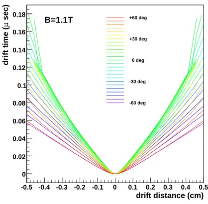
with a gap of 3 mm and the position of the sense wires are staggered. Green horizontal lines show the cathode pads. . . 43 2.16 Field map and drift lines calculated by GARFIELD simulation with the
nom-inal operated condition in MEG. . . 43 2.17 . . . 45 2.18 Timing counter bars covered with fibers for z position measurement. . . . 46 2.19 Schematic of DRS principle. . . 47 2.20 Illustration of the trigger system. . . 49 2.21 Illustration of the full programming chain for the analysis and the MC
simulation in MEG. . . 50 2.22 Number of stopped muons on the target during physics data taking of
2009–2011. . . 53 3.1 (a) An example of a PMT raw waveform from the waveform digitizer. (b)
An example of a waveform with high-pass filter. . . 55 3.2 An example event with pileup gamma ray which is identified by using the
distribution of the light yield. Magenta circles show the pileup cluster. . 57 3.3 An event with pileup which identified by the peak search. Left plot shows
the normal waveform after moving-average and right plot shows the differ-ential one. Magenta stars show the found peaks. . . 58 3.4 An waveform as same event as shown in Fig. 3.3 before (left) and after
(right) applying the pileup elimination. . . 58 3.5 Two dimensional scatter plot of the charge ratio on the inner/outer faces
vs the gamma ray interaction depth. Black points show the data from cosmic ray runs, and green ones shows the signal Monte Carlo events. The two blue lines show the selection criteria for the cosmic ray rejection. . . 59
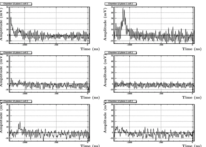
using the Garfield simulation. . . 63 3.9 Example of DCH waveforms in a cell which taken in the 2011 noisy run
period. . . 64 3.10 Example of DCH waveforms taken after hardware investigations. . . 65 3.11 Power spectrum of accumulated DCH waveforms taken in the 2011 noisy
run period. . . 66 3.12 Raw DCH waveform (black solid line) and after the filtering (red solid line)
in noisy run (a). The charge integration is done for the area between 2 blue solid lines. (b) is the power spectrum of waveform (a) before/after filtering (black/red). . . 67 3.13 A positron trajectory fitted by using the previous track fitting in an event. 70 3.14 Differences of reconstructed hits by using new/old Kalman in X-Y view
(left) and X-Z view (right). Red stars show the hits reconstructed by using new Kalman and blue ones show those reconstructed by using old Kalman. Magenta circles in the left plot shows measured hits belonging to the reconstructed track and the radius of each circle shows the measured drift distance. Black points shown in the left plot represent the position of wires. . . 71 4.1 BGO (NaI) mover(a) and two dimensional plot of gamma ray energies
measured by the LXe detector and the BGO detector(b). . . 75 4.2 Reconstructed positions of 25 α sources inside the LXe detector. In this
particular run, the half of the detector was filled with liquid xenon and the other part was filled with gaseous xenon. . . 77 4.3 Upper plot shows the light yield history measured by using CW-Li peak
(black) and background scale (red). To calibrate the light yield history, other possible sources (CEX 55 and 83 MeV gamma, 9 MeV gamma with neutron generator, cosmic-ray, and alpha source peak) are used. Combined history curve is also shown in this plot with a gray curve. Bottom plot shows same history after the correction by using the combined curve so that it becomes flat. . . 79 4.4 Correlation between za and the cathode vernier pad asymmetry (black
markers), fitted by a sinusoidal function (red line). . . 80 4.5 Corner cubes mounted on the downstream side of the drift chambers. . . 81 4.6 3D view of 10 cosmic-ray counter bars (shown in cyan). Green line shows
a simulated cosmic-ray, which pass through both drift chambers and the cosmic-ray counter. . . 82 4.7 Reconstructed positron vertex distribution in Z-Y plane in 2011. . . . 83 4.8 An illustration of the software target alignment with Michel positrons in
5.4 A Ee distribution from the data taken in 2011 with a fitting result by
using Eq. (5.6). Dashed blue line shows a resolution function centered at 52.8 MeV. Dashed black line is the theoretical Michel spectrum. In the bottom plot, the acceptance function is shown. . . 92 5.5 Differences of φe(a), θe(b), ye(c) and ze(d) between two turns from 2011
data fitted by the double Gaussian function. . . 93 5.6 Relative time distribution from 2011 data. . . 96 5.7 Residuals of the single hit z-position with/without the noise reduction. . 97 5.8 Ee spectrum in 2011 noisy run period. Red/black lines are with/without
the noise reduction. Right figure shows the log scale of the left figure. . . 99 5.9 Distributions of ∆x(x = Ee, φe, θe, ye, ze) from two-turn events in 2011
noisy run period. Red/black lines are with/without the noise reduction. . 100 5.10 Eespectrum in 2009–2011 combined data. Red/black lines are
with/with-out the noise reduction. Right figure shows the log scale of the left figure. 101 5.11 Distributions of ∆x(x = Ee, φe, θe, ye, ze) from two-turn events in 2009–
2011 combined data. Red/black lines are with/without the noise reduction. 101 5.12 Reconstructed energy spectrum of positrons with new track fitting (red)
in comparison with that with the previous one (dashed black line). Both spectra are normalized by using the area of each histogram. . . 102 5.13 Energy spectra of gamma rays in comparison between that by applying new
pileup elimination algorithm (red), previous algorithm (blue-dot-dashed) and without the pileup elimination (black-dotted). . . 103 6.1 Two dimensional event distribution in teγ vs Eγ taken in 2009–2011. The
blank box at the center shows the blind box and the inner box with blue lines shows the analysis region. Left and Right boxes with dashed black lines show the sideband data and two boxes with solid magenta lines show the time sidebands which are used for the maximum likelihood fit. A bot-tom center box shows the energy sideband used to evaluate the expected number of RMD events and the teγ resolution. For the illustration
pur-pose, following loose cuts are applied;40 ≤ Ee ≤ 60 MeV;40 ≤ Eγ ≤
60 MeV;|θeγ| ≤ 200 mrad; |φeγ| ≤ 200 mrad;|teγ| ≤ 4 ns. . . 107 6.2 Two dimensional event distribution in θeγ vs φeγ taken in 2009–2011 in
time sidebands. The center box with blue lines shows the analysis re-gion in relative angles. Neighboring four boxes with dashed lines show the angle sidebands which we perform the maximum likelihood fitting. For the illustration purpose, following loose cuts are applied;40 ≤ Ee ≤ 60 MeV;43≤ Eγ ≤ 60 MeV;|θeγ| ≤ 200 mrad; |φeγ| ≤ 200 mrad;|teγ| ≤ 4 ns
extracted from the MC distribution of RMD and AIF, Blue line show that convolved with resolution and pedestal, namely acceptance. Solid black line is contribution from cosmic-ray background and Red one shows sum of the blue one and black one. . . 119 6.6 Average PDFs for the 2009–2011 combined dataset. The green, red and
magenta lines show the signal, RMD and BG PDFs, respectively. The correlations between the errors of positron observables are corrected except for (f). . . 121 6.7 Examples of per-event PDF in typical two events observed in the time
sideband. (a) shows PDFs in which the positron-track shows good fitting quality. (b) shows ones in the event with worse fitting quality. Green lines show the signal PDFs, Magenta dashed lines show the accidental background PDFs and red lines show the RMD PDFs. Blue lines are sum of those three PDFs and black stars indicate measured variables. . . 122 6.8 (a) Average distributions of Ee (left), θeγ (center) and φeγ (right) of the
full-MC (black markers) and the toy-MC (blue solid line). (b) Average correlations of δEe v.s. δφeγ (left) and δθeγ v.s. δφeγ of the full-MC (black
markers) and the toy-MC (blue markers). . . 124 6.9 (a) Distribution of MC signal events on vertex-angle plane. Missing-turn
events make a characteristic pattern on this plane appearing as a band parallel to the red arrow. (b) Scatter plot of the MC events on teγ v.s. a new
variable defined by the projection along the red arrow in (a). The missing turn events ranging at the negative teγ are clearly distributed around −28
on the new variable. (c) and (d) show the projected distributions of MC and data (2011), respectively. Fraction of the peak events is estimated by fitting a Gaussian and a quartic function to the distribution and results are shown in (c) and (d). . . 126 6.10 Distribution of RMD events in 2009–2010 data. Black dots show the
mea-sured distribution. Black solid histograms show the expected distribution calculated from the normalization factor from Michel channel and the best estimate value for each parameter, and the gray bands show the uncer-tainty. Red dashed ones show the distribution with the best-fit values of normalization and systematic parameters. . . 129 6.11 Distribution of RMD events in 2011 data. Black dots show the measured
distribution. Black solid histograms show the expected distribution cal-culated from the normalization factor from Michel channel and the best estimate value for each parameter, and the gray bands show the uncer-tainty. Red dashed ones show the distribution with the best-fit values of normalization and systematic parameters. . . 130
the results of the positive ones. . . 135 7.3 Event distributions in Eγ v.s. Ee and teγ v.s. cos Θeγ. Corresponding
datasets are 2009-2010 combined (a)(b) and 2011 only (c)(d), respectively. The signal two-dimensional PDFs are superimposed as contours at 1, 1.645, 2 σ as blue dashed, solid, and dotted lines respectively. . . . 138 7.4 Event distributions in the (Ee, Eγ) plane(a) and (cos Θeγ, teγ) plane(b).
Corresponding dataset is 2009-2011 combined. Definition of blue contours are same as those in Fig. 7.3. . . 139 7.5 Likelihood fit result for 2009–2010 combined dataset in the analysis region.
Black markers show the data. Red and pink lines show the best fit for RMD and BG, respectively. Green line shows the best fit for the signal (almost invisible because of the small Nsig) and blue one shows total best fit. . . . 140
7.6 Likelihood fit result for 2011 dataset in the analysis region. The definitions of each components are the same as in Fig.7.5. . . 140 7.7 Likelihood fit result for 2009–2011 combined dataset in the analysis region.
The definitions of each components are the same as in Fig.7.5. . . 141 7.8 Profile likelihood curves . . . 141 7.9 Confidence level curves (a)–(c) before normalization and (d) after
normal-ization. (a) 2009-2010, (b) 2011, (c)(d) 2009-2011. . . 142 7.10 The average signal and background PDFs for the 2011 dataset. The
pa-rameters are randomized for each curve according to their uncertainties. Dark green (blue) lines are the signal (BG) PDFs without randomizing parameters and green (cyan) lines are PDFs with randomized parameters. 144 7.11 Difference of reconstructed teγ (upper left), Ee (upper center), Eγ (upper
right), θe (bottom left) and φe (bottom center) in the 2009–2010 data with
the old and the new reconstruction algorithms. The definition of ∆x is as follows:∆x = xnew− xold. . . 147
7.12 Distribution of ∆Nsig upper limits. The black arrow shows the observed
difference in the 2009–2010 combined dataset. . . 148 7.13 3D view of reconstructed events which have the first(a) and second(b)
largest Rsig value. . . 148
7.14 Event-by-event comparison for five high rank events found in new/previous analysis shown by red/black markers. Numbers represent the event of Rsig
ordering. The signal two-dimensional PDFs are superimposed as contours at 1, 1.645, 2 σ as blue dashed, solid, and dotted lines respectively. . . . 149 7.15 (a) shows B(µ→ eγ) v.s. B(τ → µγ) correlation (Fig. 1.3 in Sec. 1.2.2
[16]) with the new upper limit of B(µ+ → e+γ). (b) shows B(µ → eγ)
v.s. muon g-2 correlation (Fig. 1.5 in Sec. 1.2.3 [20]) with the new upper limit of B(µ+ → e+γ). . . . 150
A.1 Extraction of the δφev.s. δEeand δyev.s. δEecorrelations. The red vertical
line shows the target intersection with the transverse plane passing from the muon decay point V = (X, Y ). . . . 157 A.2 Extraction of the δθe v.s. δze correlation. . . 158
1.4 Recent the most stringent experimental limits given by the BABAR and
Belle experiments. Only four famous decay modes are shown here. . . 30
2.1 Several characteristics of LXe in comparison with other scintillators. . . . 35
2.2 Characteristics and Parameters of DCH. . . 44
2.3 Various trigger settings used in the MEG experiment and the prescaling factors in physics run. Approximately QL ∼ 30 MeV,QH ∼ 40 MeV,TN ∼ 20 ns and TW ∼ 40 ns. DM represents the direction-match algorithm given by the trigger. . . 48
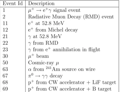
2.4 List of some important events which are prepared in MEGMC. . . 50
4.1 Several calibration and monitoring methods prepared for the LXe detector. 74 5.1 Single hit resolutions of core/tail in each year. . . 90
5.2 Performance comparison in 2009. . . 98
5.3 Performance comparison in 2010. . . 98
5.4 Performance comparison in 2011 noisy run period. . . 99
5.5 Performance comparison in 2011 run after hardware investigations. . . . 100
5.6 Performance comparison for 2009-2011 all combined data. . . 100
5.7 Performance summary. . . 104
6.1 Parameters for positron energy response. Since errors on all variables are implemented as a covariance matrix in the PDF, they are not shown in this table. . . 112
6.2 Sigmas of pulls for positron angular and vertex responses. . . 113
6.3 Parameters for the correlations and their uncertainties. . . 114
6.4 Breakdown of analysis efficiencies . . . 125
6.5 Michel normalization parameters for 2009 data in comparison with the previous estimation . . . 127
6.6 Michel normalization parameters for 2010 data in comparison with the previous estimation . . . 128
7.5 Angle sideband results without constraints on the number of backgrounds (Uncertainties are in 1σ). Parameters in bracket show the expected number of backgrounds and those with a hat show the best fit results. . . 137 7.6 Expected number of background events and the observed number of events
in the analysis region defined in Sec.6.1.3. . . 137 7.7 The best fit number of events and the corresponding branching ratios. The
uncertainties are MINOS (i.e. profile likelihood ∆NLL method) 1.645σ errors. The numbers with hats show the best fit values. . . 139 7.8 Confidence intervals (upper limits and lower limits if they are set) on the
2009-2010, 2011 and 2009-2011 datasets calculated from confidence level curves shown in Fig.7.9(d). The numbers in the first table are written in
Nsig and those in the second are in B × 1013. A confidence level at 0 is
shown only when ˆNsig is positive. The results are including the systematic
uncertainties. . . 143 7.9 Uncertainties associated to the drift chamber alignment and the magnetic
field. . . 143 7.10 Relative contributions of uncertainties to upper limit ofB in RMS of ∆∆NLL.145 7.11 Relative contributions of the uncertainties of the correlations in the positron
observables to the upper limit of B in RMS of ∆∆NLL. . . 146 7.12 Results from category PDF and comparison without systematic uncertainties.146 7.13 Detector performance which were written in the proposal and those
that cannot be explained by the SM, for example the tiny masses of neutrinos and the existence of dark matter which is the most dominant component and yet unknown matter in our universe. It clearly indicates the existence of new physics beyond the SM (BSM). In the fermion sector, it is found that there are three generations in quark and lep-ton sectors as well so-called “Flavor” and the flavor mixing was found in the quark sector which is taken into account by the CKM matrix. In the recent decade, the fla-vor oscillation in the neutrino sector called “neutrino oscillations” was also confirmed by various experiments, e.g. Super Kamiokande, Daya Bay and T2K. Therefore, the lepton flavor violation in the charged lepton sector (CLFV) has only been undiscovered yet. The µ+ → e+γ decay is one of the simple and famous decay modes of the muon
CLFV processes. In the SM framework, CLFV processes are strictly forbidden and even if non-zero neutrino mixing is considered, the branching fraction of the µ+ → e+γ
de-cay is calculated to be ∼10−50. On the other hand, the branching fraction of CLFV processes can be enhanced in many popular BSM models, e.g. SUSY-GUT, and they predict detectable branching ratios of various CLFV processes. For example, the branch-ing fraction of the µ+ → e+γ decay is expected to be in the range of 10−11–10−15 order of
magnitude depending on the values of parameters in SUSY-GUT. From the experimental point of view, the upper limit on the branching ratio of the µ+→ e+γ decay was given
as B(µ+ → e+γ) < 1.2× 10⁻¹¹ at 90% C.L. by the MEGA experiment [2] and the value
was already close to the region predicted by the new physics. Accordingly, the search for the µ+→ e+γ decay is one of the effective probes to search for the BSM.
Aiming to search for the µ+ → e+γ decay with higher sensitivity, the MEG (Mu to
Electron Gamma) experiment was proposed by a group of Japanese and Russian physicists and approved by the research committee of the Paul Scherrer Institut (PSI) in 1999 [3] and then the international collaboration was established. The MEG experiment started the physics data taking in 2008. By using 2009–2010 combined dataset, the MEG experiment has already set the upper limit of 2.4× 10⁻¹² at 90% C.L. [4]. This means that we set a 5 times tighter upper limit than that of set by the MEGA experiment. If the µ+→ e+γ
decay is discovered, it should be an evidence of new physics. Otherwise, the result will set constraint to the region of parameters allowed in the BSM and give an important hint to investigate the unknown mechanism of the BSM. Therefore, it is important to improve
→ e
• apply offline noise filtering for the drift chamber waveform analysis, • revise the fitting algorithm for the track reconstruction of positrons,
• improve the gamma ray analysis in order to get higher efficiency and suppress the
pileup events,
• take the event-by-event fitting uncertainties on positron observables into account
in the physics analysis.
We analyze 2009–2010 data again with these improvements in order to enhance the sensi-tivity as much as possible. Owing to these efforts, the sensisensi-tivity is improved by a factor 2 by analyzing 2009–2011 combined dataset [5] in comparison with the previous result.
In this thesis, the details of the analysis procedure, analysis and calibration improve-ments, and results by using 2009–2011 combined dataset is described. In Chapter 1, the details of searching for the µ+→ e+γ decay and few related theories are introduced.
The apparatus of the MEG experiment and the details of data taking during 2009–2011 are explained in Chapter 2. In Chapter 3, the method of the event reconstruction is described. The calibration tools for the MEG experiment are introduced in Chapter 4
in detail. Chapter 5 summarizes the performance and several improvements due to the new reconstruction algorithms. In Chapter 6, details of the analysis to search for the
µ+→ e+γ decay are described. The results of the analysis are written and discussed in
it cannot explain the existence of tiny masses of neutrinos, the origin of dark matter, and the reason of the large discrepancy between electromagnetic scale (O(100) GeV) and Planck scale (O(1019) GeV) called “hierarchy problem”. Hence the SM is thought to be an approximated theory of the more fundamental nature principle. In the present elementary particle physics, the most important subject is to find out the BSM which can explain above issues. Although many experiments have searched for the evidence of the BSM up to now, it has not been discovered yet. In many of the BSMs, new symmetries are introduced and new particles are predicted by those symmetries. Since the achievable energy range of direct searches for new particles such like LHC are limited by present collider technologies, indirect searches are also effective methods because undiscovered heavy particles could exist virtually as a higher order effect. Therefore, searching for the CLFV process is one of the powerful methods to investigate the BSM. In particular, muon CLFV searches are good probes because a large amount of muon can be produced more easily than the case of the tau lepton because of its longer life time (2.2 µs). In addition, the final state of muons are simpler than those of the tau lepton because of the smaller mass of muon (mµ = 105.6 MeV). The µ+ → e+γ decay is one of the famous muon
CLFV processes. In this chapter, several decay modes of the muon in the Standard Model and those in new physics are described. Possible sources of background in searching for
µ+→ e+γ decay are also discussed.
1.1
Muon Decay in the Standard Model
The µ+ → e+γ decay has been explored for more than 50 years since the muon was
discovered in 1937 [6]. Table1.1 shows decay modes of muon and its branching fractions or upper limits. As written in this table, µ± decays into e± and two neutrinos in almost 100% probability. This decay mode is called “Michel ” decay [13] and the total lepton number is conserved in this process.
µ− → e−νeνµ < 1.2 % [10]
µ+ → e+γ < 2.4× 10⁻¹² [4]
µ+ → e+e+e− < 1.0× 10⁻¹² [11]
µ− → e−γγ < 7.2× 10⁻¹¹ [12]
1.1.1
Michel Decay
In the SM, muon decay is determined by the V − A interaction. The differential decay rate of Michel decay is given by [14]
d2Γ(µ+ → e+νeνµ) dxd(cos θ) = mµ 4π3Weµ 4 G2F √ x2− x2 0 ×(FIS(x) + Pµcos θeFAS(x)) ×(1 + ~Pe(x, θe· ˆξ)), (1.1)
where Weµ = (m2µ+ m2e)/(2me), x = Ee/Weµ and x0 = me/Weµ. Here Ee is the energy
of the e+ and me and mµ are the masses of electron(positron) and muon, respectively.
Allowed region of x is from x0 to 1 by its definition. θe is the angle between the muon
polarization ( ~Pµ) and the positron momentum, and ˆξ is the directional vector of the
measurement of the positron spin polarization. FIS(x) and FAS(x) are the isotropic and
anisotropic parts of the positron energy spectrum, respectively and they are given by [15]
FIS(x) = x(1− x) + 2 9ρ(4x 2− 3x − x2 0) + ηx0(1− x), (1.2) FAS(x) = 1 3ξ √ x2− x2 0 ( 1− x +2 3δ[4x− 3 + ( √ 1− x2 0− 1)] ) , (1.3)
where ρ, η, ξ and δ are called Michel parameters. In the SM, Michel parameters are calculated to be:
ρ = 3
4, η = 0, ξ = 1, δ =
3
4. (1.4)
1.1.2
The µ
+→ e
+γ Decay in the Standard Model
The µ+ → e+γ decay is strictly forbidden in the SM because of the law of lepton flavor
conservation. If the neutrino oscillation is considered, the µ+ → e+γ decay can happen
through the Feynman diagram shown in Fig. 1.1. However, the calculated branching fraction is approximately 10−50 and almost undetectable with any existing experimental technologies. It means that if the µ+ → e+γ decay would be discovered, it should be the
µ+ ν
µ νe e+
Figure 1.1: Feynman diagram for the µ+ → e+γ decay through the neutrino oscillation.
1.2
The µ
+→ e
+γ decay and Physics Beyond the
Stan-dard Model
Many BSMs predict that the µ+→ e+γ decay can happen in a detectable range of the
branching fraction. Here several BSMs that can enhance the branching fraction of the
µ+→ e+γ decay are introduced. The effective Lagrangian for the µ+→ e+γ decay is
given by [14] Lµ→eγ =− 4G√F 2 [mµARµRσ µνe LFµν + mµALµLσµνeRFµν+ H.c.]. (1.5)
where the term of GF is the Fermi coupling constant, AR and AL are coupling constants
that correspond to the left-handed process and right-handed one, respectively. From Eq. (1.5), the differential angular distribution of µ+ → e+γ decay is given by
dB(µ+ → e+γ)
d(cos θe)
= 192π2[|AR|2(1− Pµcos θe) +|AL|2(1 + cos θe))], (1.6)
where θe is the angle between the muon polarization and the e+ momentum vectors.
The supersymmetric (SUSY) model is one of the candidates of the BSMs, which can answer several issues in the SM. In the SUSY, new gauge symmetry called “supersymme-try” is introduced as an extension of the SM. As a result, all of elementary particles in the SM have their own supersymmetric partners called “sparticles”. Table 1.2 shows all par-ticles and sparpar-ticles which are contained in the minimal supersymmetric standard model (MSSM). If the supersymmetry is not broken, each sparticle should have the same mass of its own supersymmetric partner. However, such particles have not been discovered yet. Therefore the supersymmetry is thought to be broken. In the MSSM, the different masses between sparticles and their own partners are generated by the soft SUSY-breaking terms. As a result, the branching fractions of CLFV processes are enhanced by the flavor mixing in the slepton sector.
1.2.1
SUSY GUT SU(5)
The SUSY grand unified model (SUSY GUT) is one of attractive models of the SUSY extensions, because three gauge coupling constants of strong, weak, and electromagnetic
(×3 families) d d˜∗R d†R (3, 1, 1/3) sleptons,leptons l (˜νL ˜eL) (ν eL) (1, 2,−1/2)
(×3 families) e e˜∗R e†R (1, 1, 1)
Higgs,higgsinos Hu (Hu+ Hu0) ( ˜Hu+ H˜u0) (1, 2, 1/2)
Hd (Hd0 Hd−) ( ˜Hd0 H˜d−) (1, 2,−1/2)
Names spin 1/2 spin 1 SU (3)C, SU (2)L, U (1)Y
gluino, gluon g˜ g (8, 1, 0) winos, W bosons W˜± W˜0 W± W0 (1, 3, 0) bino, B boson B˜0 B0 (1, 1, 0) ˜ χ0 µ e ˜ µR e˜R ˜ χ0 e µ ˜ µR ˜ τR ˜ eR
Figure 1.2: Feynman diagrams for the µ+ → e+γ decay in SU(5) SUSY GUT.
interactions are unified to a single SU (5) gauge coupling constant at a scale of the order of 1016 GeV (called GUT scale) in the SUSY GUT. The off-diagonal elements of the
right-handed slepton mass matrix in the SUSY GUT are given by
(m2e˜ R)ij =− 3 8π2(VR)i3(VR) ∗ j3|y33u |2m20(3 +|A20|) ln ( MP MG ) . (1.7)
where VR is a matrix element to diagonalize the Yukawa coupling constant for leptons,
MP and MG represent the reduced Planck mass (∼ 2 × 10¹⁸ GeV) and the GUT scale
(∼ 2 × 10¹⁶ GeV), respectively. Here m
0 is the universal scalar mass and A0 is the
universal trilinear coupling. As a result, Eq. (1.7) becomes a source of the µ+→ e+γ
decay. Figure 1.2 shows possible Feynman diagrams for the µ+→ e+γ decay in SUSY
GUT. In the SU (5) SUSY GUT, CLFV processes appear only in the right-handed slepton sector because of moderate values of tan β, which is defined by the ratio of two Higgs vacuum expectation values (tan β ≡ hH0
2i/hH10i). Therefore only µ+ → e
+
Rγ decay is
Figure 1.3: Correlation between B(µ→ eγ) and B(τ → µγ) as a function of mN 3, for
constraint MSSM assuming universality of the soft-SUSY breaking at the scale of gauge coupling unification, MX so-called minimal supergravity (mSUGRA) framework from
[16]. Different colored regions correspond to θ13= 1
◦
, 3◦, 5◦ and 10◦ (red, green, blue and pink, respectively) and recent experiments report the large value of θ13∼ 10
◦
[17]. Dashed line labeled “MEG2011” is added to the original plot and it represents the 90% C.L. upper limit given by the previous result of MEG [4].
1.2.2
SUSY Seesaw
In the SUSY seesaw model, right-handed heavy Majorana neutrinos are introduced to explain the tiny masses of neutrinos by the seesaw mechanism. By including the seesaw mechanism in the SUSY standard model, the right-handed neutrino supermultiplets, the Majorana mass matrix and a new Yukawa coupling constant matrix are included in the part of the lepton sector Lagrangian. Because of the presence of the Yukawa coupling constant matrix for the neutrino sector as same as the charged lepton sector, the lepton flavor would no longer be conserved separately for each generation in the SUSY seesaw. Hence the branching fractions of CLFV processes are expected to be enhanced. If we assume that the neutrino mixing mostly originates from the neutrino Yukawa coupling constants, (yν)ij, the branching ratios from µ+ → e+γ and τ → µγ
decays can be evaluated by using the neutrino mixing parameters. Figure 1.3 shows the scatter plot of the correlation between B(µ→ eγ) and B(τ → µγ) in an example of the SUSY model which including the large mass of right-handed Majorana neutrino. In this model, the µ+ → e+γ decay can happen in somewhere experimentally achievable range.
while the theoretical calculation with the SM is given as [19]:
aSM= 11 659 184(6)× 10−10 (0.7 ppm). (1.9) The discrepancy between aµ and aSM is calculated to be 2.9σ.
Since both the µ+→ e+γ decay and the muon magnetic moment are generated by
dipole operators as shown in Fig.1.4, the branching ratio of the µ+→ e+γ decay correlates
to the value of ∆aµ= (gµ− gµSM)/2 if ∆aµ is generated by the contribution from the new
physics [20]. For example, the B(li → ljγ) can be expressed by using ∆aµ as
B(li → ljγ) B(li → ljνliνlj) = 48π 3α G2 F ( ∆aµ m2 µ )2 × ( f2c(M22/M˜l2, µ2/M˜l2) g2c(M2 2/M˜l2, µ2/M˜l2) ) |δij LL| 2, (1.10)
where µ is the supersymmetric-invariant mass term of the Higgs potential, M˜l is a mass
of left-handed slepton, , f2c(x, y) and g2c(x, y) are defined as
f2c(x, y) = −x2− 4x + 5 + 2(2x + 1) ln x 2(1− x)4 − −y2− 4y + 5 + 2(2y + 1) ln y 2(1− y)4 , g2c(x, y) = (3− 4x + x2+ 2 log x) (x− 1)3 − (3− 4y + y2+ 2 log y) (y− 1)3 , (1.11)
in the MSSM extension with the seesaw mechanism. Here δLLij is the left-handed slepton mass matrices read as
δijLL = cν(yν†yν)ij, (1.12)
where cν is a numerical coefficient. Figure1.5shows correlation between the B(µ+ → e+γ)
and ∆aµincluding the non-linear effect not shown in Eq. (1.10). Therefore if the reported
(g − 2)µ anomaly is really exist, the branching ratio of the µ+ → e+γ decay might be
enhanced. Otherwise, there should be some mechanism which can suppress the lepton flavor violation. Consequently, both the measurement of the muon magnetic moment and the µ+ → e+γ decay search play the important roles to find out the unknown mechanism
of new physics.
1.3
Searches for the CLFV Processes
1.3.1
Experimental History of the µ
+→ e
+γ Decay Searches
Recent results from experimental searches for the µ+→ e+γ decay are shown in Table1.3.
Before starting the MEG experiment, the best upper limit on the µ+ → e+γ decay was set
to be 1.2×10⁻¹¹by the MEGA experiment. The MEG experiment already achieved more stringent upper limit by using 2009–2010 combined dataset in 2011. As already discussed, the B(µ+→ e+γ) is expected to be within 10−11–10−15 in several BSMs. According to
the upper limit given by the previous result in the MEG experiment, we already achieved the sensitivity which is able to explore the new physics.
µ e µ µ
Figure 1.4: Simplified Feynman diagram of the µ+→ e+γ decay (left) and the muon
magnetic moment (right).
Figure 1.5: Correlation between B(µ+→ e+γ) and ∆aµfrom [20]. Horizontal dashed line
labeled “MEG2011” is added to the original plot and it represents the 90% C.L. upper limit given by the previous result of the MEG experiment. Vertical two dashed lines are also added and they represent the 1σ region of the (g − 2)µ anomaly measured in the
E821 experiment [18]. Assumed parameters are as follows;|δ12
LL| = 10−4, |δLL23| = 10−2.
Here the relatively small slepton mass and large tan β are assumed. The inner red area satisfy the B-physics constraints.
(Hz) (%) (%) (ns) (mrad) 90% C.L. 1977 SIN 5× 10⁵ µ+ 10 8.7 6.7 1.0× 10⁻⁹ [22] 1977 TRIUMF 2× 10⁵ π+ 8.7 9.3 1.4 3.6× 10⁻⁹ [23] 1979 LAMPF 2.4× 10⁶ µ+ 8.8 8 1.9 37 1.7× 10⁻¹⁰ [24] 1986 LAMPF 4× 10⁵ µ+ 8 8 1.8 87 4.9× 10⁻¹¹ [12] 1999 LAMPF 1.3× 10⁷ µ+ 1.2 4.5 1.6 15 1.2× 10⁻¹¹ [2] 2011 PSI 3× 10⁷ µ+ 1.6 4.7 0.35 30 2.4× 10⁻¹² [4]
1.3.2
Background
Two different types of background sources are considered in the search for the µ+→ e+γ
decay. First one is the radiative muon decay (RMD) which is called “prompt background”. In RMD, a muon decays into two neutrinos, a positron and a gamma ray. Since there are two invisible particles in the final state, it can be misidentified as a signal event if both a positron and a gamma ray have high energy close to 52.8 MeV. The other is the accidental background (BG) which is the most dominant one in recent µ+→ e+γ
search experiments. In the accidental background, a gamma from RMD, annihilation in flight (AIF) of a positron, or bremsstrahlung of a positron accidentally overlaps with a positron from Michel decay. In the MEG experiment, RMD and AIF are main sources of the background gamma ray and the fractions are found to be nearly equivalent from a simulation study. Here the details of each background source are explained and the background situation in the MEG experiment is discussed.
1.3.2.1 Prompt Background
The decay of RMD can be written as µ+ → e+ν
eνµγ. If two neutrinos carry only a
small amount of energy, the opening angle between e+ and γ ray becomes close to 180◦.
Moreover, the e+ and the γ have approximately the same energy as in signal event in this case. The decay width of RMD, dΓ(µ→ eννγ) is given by
dΓ(µ→ eννγ) = G 2 Fm5µα 3× 28π4 × [ (1− x)2(1− Pµcos θe) + ( 4(1− x)(1 − y) − 1 2z 2 ) (1 + Pµcos θe) ] ×dxdyzdzd(cos θe), (1.13)
where θe is the opening angle between the muon spin and the positron direction, x =
J1 = 3(δx) (δy) 2 − 2(δx) 2 +3(δy)2 2 , (1.15) J2 = 8(δx)2(δy)2 ( δz 2 )2 − 8(δx)(δy) ( δz 2 )4 +8 3 ( δz 2 )6 , (1.16)
where δx, δy and δz are half-widths of the signal region for x, y and z, respectively. Here Γ(µ→ eνν) is the total muon decay width and Eq. (1.15) and Eq. (1.16) are deter-mined by assuming δz ≤ 2√δxδy and this assumption fits into the situation of the MEG
experiment. In case fully depolarized muon, Eq. (1.14) read as
dB(µ → eννγ) = α
8π[J1+ J2]. (1.17) For example, we can calculate the effective branching ratio with Eq. (1.17) in the situation of the MEGA experiment by using numerical numbers written in Table 1.3 by keeping signal efficiency to be 90% as;
δx = 0.0084, δy = 0.032, δz = 0.021, δteγ = 1.12 ns. (1.18)
By using these numbers, the branching ratio of the prompt background is given as,
B(µ→ eννγ) ∼ 4.4 × 10⁻¹⁵. (1.19)
Therefore the prompt background is negligible in recent µ+→ e+γ search experiments.
1.3.2.2 Accidental Background
The accidental background is the most dominant background to search for the µ+→ e+γ
decay in the recent experiments including MEG. The effective branching fraction (Bacc)
is given by Bacc= Rµ· fe0· f 0 γ · ( dωeγ 4π )· (2δteγ), (1.20)
where Rµ is the instantaneous muon intensity, the back-to-back resolution (dωeγ/4π) is
given by (dωeγ/4π) = (dz)2/4, fe0 and fγ0 are integrated spectra of background gamma
rays and positrons within the signal region, respectively. Therefore the excellent angular and gamma energy measurements are required to suppress the accidental background. The factor f0
e can be approximately estimated to be ≈ 2(δx) by integrating Michel
spectrum over 1− δx ≤ x ≤ 1 since it is almost flat at x ' 1 as shown in Fig. 1.6(a). In order to make a situation simpler, f0
γ is assumed to be dominated by the RMD events
and muons not to be polarized. In this case, f0
γ is given by fγ0 = ∫ 1 1−δy dy ∫ d(cos θγ) dB(µ → eννγ) dyd cos θγ ≈ (α 2π ) (δy)2[ln(δy) + 7.33]. (1.21)
Normalized Positron Energy (x)
0 0.2 0.4 0.6 0.8 1
Differential Branching Ratio
0 0.2 0.4
(a)
Normalized Gamma Energy (y)
0 0.2 0.4 0.6 0.8 1
Differential Branching Ratio
-7 10 -6 10 -5 10 -4 10 (b)
Figure 1.6: Left figure shows positron energy spectrum of unpolarized µ+ → e+ν
eνµdecay
(Michel spectrum). A radiative decay correction [25] is included. Right one shows gamma Energy spectrum of unpolarized µ+ → e+νeνµγ decay. Positron energy and the angle
between a positron and a gamma are integrated.
From Eq. (1.20), the branching fraction of the accidental backgrounds is proportional to
Rµ.
A gamma ray from annihilation-in-flight (AIF) of a positron is other possible source of the accidental background. The energy spectrum and the production rate of the gamma ray from AIF depends on the materials inside the tracking volume. The rate of the AIF background is also proportional to the instant muon rate (Rµ) since almost all positrons
originate from Michel decay of muons.
By way of example, the branching ratio of the accidental background is calculated by using resolution parameters given by the MEGA experiment. In the calculation, it has to be considered that pulsed muon beam was used in the MEGA experiment. The instant beam intensity was 2.6× 10⁸ in MEGA. The effective branching ratio is given as
Bacc∼ 2.4 × 10⁻¹². (1.22)
Therefore the accidental background was dominant in their experiment and it could be a serious problem on searching for the µ+→ e+γ decay with higher sensitivity of 10−13
level.
1.3.2.3 Experimental Requirement for the µ+→ e+γ Search
As discussed in above sections, it is the most important to reduce the accidental back-ground to achieve the sensitivity below 10−12. Since the background rate is proportional to an instant muon rate, direct-current (DC) muon beam is strongly preferred in order to suppress the accidental background while keeping the total statistics high enough.
Since the incident rate of the AIF background depends on the materials along the positron trajectories, namely the target and the tracking devices, the total amount of materials inside the tracking volume should be as small as possible and they should be
gamma ray. This method helps to achieve the 4.5% precise energy measurement in FWHM, however it causes the trade-off effect of the low detection efficiency which was measured to be 2.4% in MEGA. Consequently, the single event sensitivity was limited in their experiment. In order to achieve the sensitivity less than 10−12, the same level of the energy resolution for gamma rays as MEGA with much higher detection efficiency is required for the gamma ray detector.
1.3.3
Comparison with Other CLFV Searches
Here some of other CLFV processes and related experimental searches are described together with the associated models of new physics for comparisons. The µ+ → e+e+e−
decay and the µ−− e−coherent conversion are promising channels to search for the BSM as same as the µ→ eγ decay by using muons. As one can easily imagine, the branching fraction of those two processes are strongly correlated to that of the µ+ → e+γ decay.
In case of the µ+ → e+γ decay, contributions for the effective Lagrangian are dominated
by photon-penguin diagrams as shown in Fig. 1.2. On the other hand, those of the
µ+→ e+e+e− decay and the µ−− e− conversion are enhanced by mediating the direct
four-fermion interactions and the contributions from the photonic interactions of these processes are relatively small due to an additional coupling between a gamma line and a fermion line in the Feynman diagrams. Here each of muon CLFV processes are briefly discussed together with the relation to the µ+→ e+γ decay and the experimental aspects.
1.3.3.1 µ+ → e+e+e− decay
If only photon-penguin diagrams contribute to the µ+→ e+e+e−decay, a model-independent branching ratio of µ+ → e+e+e−can be derived by using the branching ratio of µ+ → e+γ,
as follows [14]: B(µ+ → e+e+e−) B(µ+→ e+γ) ' α 3π [ lnm 2 µ m2 e − 11 4 ] = 0.006. (1.23)
The signal event can be well identified by using following two requirements:
• The conservation of momentum (|∑i~pi| = 0) and energy (
∑
iEi = mµ),
• Timing coincidence between two positrons and one electron.
For the µ+→ e+e+e−decay search, two main background sources are considered. One is a prompt background; µ→ e+e+e−ν
eνµ, which is allowed in the SM and can be a fake
of the signal event, when two neutrinos have tiny energies. The branching ratio of this decay is (3.4 ± 0.4) × 10−5 [9]. The other background is an accidental coincidence of an e+ from normal muon decay with an uncorrelated e+e− pair, for example, produced
→ e
One experiment, aiming to search for the µ+→ e+e+e− decay with 104 times higher
sensitivity than the present upper limit, was proposed in PSI [26]. They proposed a staged approach in the sensitivity to BR∼ 10−15 in phase I and further improvements to BR∼ 10−16 at later stages if a new high-intensity muon beam (HiMB), which is a future planned beamline at PSI, is realized. If the photonic contributions are dominant, the current upper limit corresponds to the 10−10 order of magnitude of that for the
µ+→ e+γ search and the goal sensitivity of proposed new experiment corresponds to
10−14 level.
1.3.3.2 µ−− e− Conversion
In the SM, a negative muon, which is captured by an atom and forms muonic atom, can either decay in an orbit (µ− → e−νµνe) or is captured by a nucleus of mass number A
and atomic number Z, namely,
µ−+ (A, Z)→ νµ+ (A, Z− 1). (1.24)
However, the µ−− e− conversion in a muonic atom, such as
µ−+ (A, Z)→ e−+ (A, Z), (1.25) is expected to occur in the BSM, which violates the conservation of the lepton flavor num-bers as same as in the µ+ → e+γ decay. From here, the µ−− e− conversion is expressed
as µ−N → e−N . Similar to Eq. (1.23), the ratio of B(µ+ → e+γ)/B(µ−N → e−N ) is
given by [14] B(µ−N → e−N ) B(µ+ → e+γ) = G2Fm4µ 96π3α × 3 × 10 12B(A, Z)∼ B(A, Z) 428 , (1.26) where only the photonic contributions are assumed and B(A, Z) represents the factor depending on the mass number (A) and the atomic number (Z) of the target nucleus. For example, for the titanium nucleus, the values of B(A, Z) is calculated to be 1.8– 2.2, based on different approximations. Therefore, the ratio of B(µ−N → e−N ) and
B(µ+→ e+γ) is calculated to be B(µ−N → e−N )/B(µ+→ e+γ)∼ 0.0042–0.0051. In the
muonic atom, most muons transit to the ground state before decaying or being captured by the nucleus. Therefore if µ−− e−would happen, the energy of emitted electron should be monochromatic as
Eµe= mµ− Bµ, (1.27)
where Bµ is the binding energy of the 1s muonic atom. Since the value of Bµ is different
for various nuclei, the peak energy of the µ−− e− conversion signal also changes, for example, Eµe = 104.3 MeV for titanium. Event signature is very simple that, only one
introduced below. A radiative pion capture (π−+ (A, Z)→ (A, Z − 1) + γ) could be one of the background sources. However, they can be suppressed by reducing the amount of pions which reach the muon target by using long enough muon transport solenoid. Other backgrounds could be caused by the decay in flight or interactions of particles (muon, pion, (anti)proton) in a primary proton beam. Since the muonic atoms have lifetimes of the order of 1 µs, the beam origin backgrounds can be suppressed by using high-intensity pulsed beam when the measurements are only done during the beam intervals. In this case, the purity of the pulse, which called “extinction”, is essential since the remaining particles between two pulses could make the background.
The current upper limit was set by the SINDRUM-II experiment at 7×10⁻¹³(90% C.L.) [21], which used the negative DC muon beam at the πE5 area in PSI.
In near future, two different experiments are being prepared to search for the µ−− e− by using high-intensity pulsed beam at the different places. One is the Mu2e experiment at Fermilab [27] and the other is the COMET experiment at J-PARC [28]. The goal sensitivities of both experiments are similar, at 10−16level. Since the present upper limit and the goal sensitivity are similar to those of µ+ → e+e+e− search, similar calculation
can be done for the µ−− e− conversion as well.
For both the µ+ → e+e+e− decay and the µ−− e− conversion searches, the branching
fractions could be expected to be enhanced if some other contributions are considered. For example, in the little higgs model with T-parity, the lepton flavor violation can be happen through the additional mirror sector and the lepton flavor is not conserved any more [29]. In this model, the ratios between different three processes become comparable as namely B(µ→ eγ) ∼ B(µ → eee) ∼ B(µ − e). Accordingly, the more information about the new physics can be obtained by comparing the results of different three CLFV modes.
1.3.3.3 CLFV in τ decay
Here, four CLFV decay modes of tau lepton are briefly described. The experimental searches for CLFV processes of tau lepton channel are done by using those generated by colliders since the tau lepton beam cannot be produced by present technologies because of its extremely shorter lifetime (0.29 ps) compared to that of muon. Current upper bounds are given by BABAR and Belle as shown in Table1.4. In the near future, Belle-II collaboration aiming to search for the tau LFV with higher intensity electron positron collider. The LHCb experiment will also search for the tau on CLFV processes by using the Large Hadron Collider.
Table 1.4: Recent the most stringent experimental limits given by the BABAR and Belle experiments. Only four famous decay modes are shown here.
Mode 90% upper limit Experiment
B(τ → µγ) 4.4× 10⁻⁸ BABAR[30]
B(τ → eγ) 3.3× 10⁻⁸ BABAR[30]
B(τ → µµµ) 2.1 × 10⁻⁸ Belle[31]
a sensitivity goal of 10 . The experimental proposal was submitted to the science committee of PSI in 1999 and the MEG collaboration was established in collaborating with 50–60 scientists from the institutes in Japan, Switzerland, Italy, Russia and United States. Dedicated detectors were constructed in order to achieve the sensitivity goal for the µ+ → e+γ search [32]. The MEG detector is placed in the πE5 area in which the world
most intense Direct-Current (DC) muon beam is provided by the proton ring cyclotron at PSI.
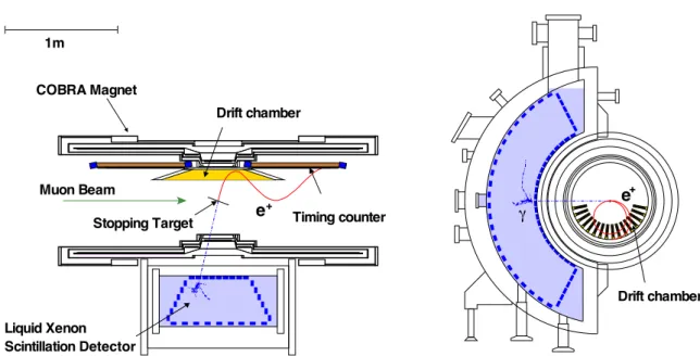
The schematic views of the MEG experiment and the global experimental coordinate is shown in Fig.2.1and Fig.2.2. The center of the coordinate is set a origin at the center of the magnet. Other coordinate expressions as follows are used as well:
r =√x2+ y2, φ = tan−1(y/x), θ = tan−1(r/z), z = z, (2.1)
with a same origin of the (x, y, z) coordinate. For gamma ray measurement, an innovative detector using large volume liquid xenon (900 litters), which works as a total absorption calorimeter, was developed and scintillation photons are read by surrounding 846 Photo Multiplier Tubes (PMTs) to determine the timing, the position and the energy of incident gamma rays. In order to reconstruct the track of positrons, a set of drift chambers built with very low mass materials are used inside a superconducting magnet which has a specially designed gradient magnetic field. At each end of the magnet warm bore outside the drift chambers, 15 plastic scintillating bars are placed to measure the impact time of positrons in several tens ps of precision. For the data taking, we use fast waveform digitizers together with the trigger system consists of Flash Analog-to-Digital Converters (FADC) and a Field Programmable Gate Array (FPGA) system.
This chapter describes the details of the experimental apparatus, the analysis method, and the run conditions in 2009, 2010 and 2011 data taking.
2.1
Beamline
In order to get a high intensity DC muon beam, the proton ring cyclotron located at PSI is a unique choice for the MEG experiment, because it can provide the world most powerful
Figure 2.1: Top and side view of all the experimental apparatus with coordination.
Figure 2.3: 590 MeV proton ring cyclotron at PSI.
2.1.1
Muon Beamline
In order to avoid muons to form the muonic atoms with materials inside the target, a positive muon (µ+) is adopted for the experiment. At the πE5 beamline, a positive muon beam is delivered from the main proton ring cyclotron.
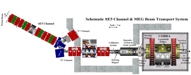
In the upstream of the πE5 beamline, muons only from pions decaying at the surface of the pion production target (E-target), are collected (so-called “surface muon”) and they are delivered to the MEG detector as shown in Fig. 2.4.
Therefore, almost all muons are fully polarized and have almost same momenta of 28 MeV/c with 5–7% of spread in FWHM (Full Width at Half Maximum). Because of the smaller momentum spread, high purity and high intensity muons are selectable. A large contamination of positrons are separated by using both electric and magnetic fields in a Wien filter with a 8.1σ separation. The low momentum of the surface muon allows to use the thin target to stop muons, which is important to suppress the production of the background gamma rays inside the target. Furthermore, easier modifications of the beam size and the transportation are possible because of its small momentum spread.
Since the frequency of the proton beam is high enough (50.6 MHz) compared with the decay time of pions (τπ± ≈ 26 ns) and that of muons (τµ ≈ 2.2 µs), the muon intensity is
almost continuous. At the background reduction point of view, the continuous beam is quite important as already explained in Sec. 1.3.2.2. The stopping rate at the target is tuned to be 3.0× 10⁷ µ+/s at a 2.2 mA of proton current.
2.1.2
Beam Transport Solenoid
The superconducting beam transporting solenoid (BTS) is placed to connect between the
πE5 beamline and the detector part. Since the BTS is directly couple to the beamline,
Figure 2.4: Schematic view of the πE5 beam channel including the beam transport system and detectors.
the BTS consists of iron-free cryogenics and magnets. At the central part of the BTS, a 300 µm thick Mylar degrader is placed to reduce the momentum of muons so that mostR of them can be stopped in the thin target at the center of the detector magnet with a minimum multiple scattering contribution to the beam. In order to focus the muon beam at the degrader position and inside the detector, a 0.36 T magnetic field is generated by using the double-layered iron-free coil.
2.1.3
Target
In order to get high stopping power of muons and to reduce the materials which can generate the background, the target is implemented as a 205 µm thick sheet of a low-density layered-structure of a polyethylene and polyester with an elliptical shape and placed on the center of the superconducting magnet with a 20◦slant angle along the beam axis. The length of semi-major and semi-minor axes are 10 cm and 4 cm respectively. There are six holes on the target in order to perform the software target alignment by analyzing the data as shown in Fig. 2.5(a). The target is placed at the almost center of the COBRA magnet (See Fig. 2.5(b)). At the target, the muon polarization is measured to be 89± 4% by using the angle distribution of Michel positrons and it is confirmed by analyzing RMD events [34].
2.2
Gamma Detector
With a gamma detection part, we need to detect the signal-like high energy gamma rays with a high detection efficiency. On the other hand, the background contamination must be highly suppressed. In order to realize such a kind of detector, following three points,
1. to reconstruct Eγ with an excellent resolution,
2. to measure the first conversion time of gamma rays precisely, 3. to reconstruct the first conversion point with a mm precision,
(a) (b)
Figure 2.5: Muon target (a) and installed view inside the COBRA magnet (b).
Table 2.1: Several characteristics of LXe in comparison with other scintillators.
LXe LAr NaI(Tl) CsI(Tl) BGO Density (g/cm3) 2.98 1.40 3.67 4.51 7.40 Radiation length (cm) 2.77 14 2.59 1.86 1.12 Moliere radius (cm) 4.2 7.2 4.13 3.57 2.23 Decay time (ns) 45 1620 230 1300 300 Wavelength (nm) 178 127 410 560 480 Relative light yield 75 90 100 165 21
are needed to be satisfied for the gamma detector. In the MEG experiment, a Liquid Xenon (LXe) detector is adopted as the gamma detector to fulfill those three require-ments. In this section, several properties of the LXe and the principle of the LXe detector are described.
2.2.1
Liquid Xenon
Since the LXe can realize non-segmented volume, the detector response can be more uniform than that of the detector based on segmented crystal. The faster decay time of the LXe helps to reduce the pileup probability effectively and provides good time resolution. Because of its short radiation length and high density, high detection efficiency is achievable. The characteristics of LXe are summarized in Table 2.1. Even though LXe has feasible scintillation properties to measure the energy of the gamma ray, there are mainly three difficulties to overcome as follows:
1. Low and the narrow operational temperature range between 161.4–165.1 K in order to keep the xenon in the liquid phase [7]