RHICでの核子対あたり重心系衝突エネルギー200GeVの金金原子核超周辺衝突におけるJ/ψ光生成

(1)

学位論文

J/ψ photoproduction in Au+Au

ultra-peripheral collisions at

√

_s

N N

= 200 GeV at RHIC

(RHIC

での核子対あたり

重心系衝突エネルギー

200GeV

の

金金原子核超周辺衝突における

J/ψ

光生成)

平成

25 年

12 月博士

(理学)

申請

東京大学大学院理学系研究科

物理学専攻

髙原明久

(2)

(3)

Abstract

The photo production of J/ψ in Au+Au collisions at the center of mass energy per nucleon pair of 200 GeV have been studied at the PHENIX experiment at mid and forward rapidity at Relativistic Heavy Ion Collider (RHIC) at Brookhaven National Laboratory (BNL).

For central-rapidity, the dσ/dy of J/ψ +Xn(< 2mrad) was measured to be 45.6±13.2 (stat)±

6.0 (sys) µb. The d2_σ/dydp

T of J/ψ +Xn(< 2mrad) distribution was measured and it shows

clear coherent peak and wider incoherent distribution. Additionally, the result of first measure-ment at forward-rapidity was described in the thesis. The new result shows incoherent process is dominant at the forward rapidity region.

(4)

Abstract

米国率ブルックヘブン研究所における RHIC 加速器を用いた PHENIX 実験において核子対あた り重心系エネルギー 200GeV での金金衝突における J/ψ の光合成過程を前方及び後方ラピディ

ティ領域において測定した。中心ラピディティ領域において J/ψ +Xn(< 2mrad), dσ/dy 45.6±

13.2 (stat)±6.0 (sys) µb の結果を得た。d2σ/dydpT of J/ψ +Xn(< 2mrad)分布の測定を行い、

明瞭なコヒーレントピークと広いインコヒーレント分布を確認した。

加えて前方領域については初の測定を行った。この新しい結果は前方ではインコヒーレント過程が種であると示すものである。

(5)

List of Figures

1.1 Gluon, sea and u and d valence distributions extracted by HERA-ZEUS at

Q2 =10 GeV2 [1] . . . 2

2.1 The measured F2 distributions via e+p collisions [1] . . . 7

2.2 The ratio of F2 structure functions of various nuclei to that of deuterium [5] . . 9

2.3 Left:F2 ratios for Pb versus x at fixed Q2 = 3 GeV2 from various models [12, 13,

14, 15, 16, 17, 18, 19, 20, 21]. Ratios of gluon distribution functions for Pb versus

x from diﬀerent models at Q2 _{= 5 GeV}2 _{[12, 13, 14, 15, 16, 17, 18, 19, 20, 21] .} ₁₀

2.4 Theoretical calculation of Ri [22] . . . 11

2.5 The diagram of J/ψ production. . . . 12

2.6 Left:Theoretical prediction of Rg_Au. Right:2004 UPC J/ψ +XN result with

the-oretical predictions [30, 29, 32, 33, 34, 22]. . . 13

2.7 The diagram of LT contribution and γp diﬀractive process [36]. . . . 14

2.8 Left:Theoretical prediction of Integrated over rapidity (|y| < 3) the

momen-tum transfer distributions for the J/ψ in the coherent (solid line) and incoherent (dashed line) photoproduction in UPC of Au ions at RHIC [38]. Right:Theoretical prediction of incoherent UPC J/ψ number of emitted neutron distribution

with-out any trigger requirement at √sN N = 200 GeV [38]. . . 15

2.9 Theoretical prediction of UPC J/ψ cross section distribution with any trigger

requirement at √sN N = 200 GeV. Black dots are old preliminary result, they

can be ignored. . . 16

2.10 Left:dN/dmee distribution fitted to the combination of a dielectron continuum

(exponential distribution) and a J/ψ (Gaussian) signal at √sN N =200 GeV in

the 2004 PHENIX run [30]. Right:2004 UPC J/ψ +XN result with theoretical

predictions [30, 40, 38, 41, 42, 43]. . . 17

3.1 The figure is the map of RHIC. . . 20

3.2 Left:The PHENIX beam (upper) and side (lower) view in the 2007 PHENIX run.

Right:The PHENIX beam (upper) and side (lower) view in the 2010 PHENIX

run. . . 21

3.3 The definition of the PHENIX coordinate. . . 22

3.4 (a) single BBC. (b) A BBC array. (c)The BBC is mounted on the PHENIX

beam pipe. . . 23

3.5 A:A top view of ZDC layout B:A beam view. . . 24

3.6 The ZDC inside schematic view. . . 25

(10)

3.8 The layout of PHENIX magnet. . . 27

3.9 The mapping of PHENIX magnetic field for CM+- case. . . 28

3.10 The frame of DC. . . 30

3.11 Left: The setup of DC wires in sector side view. Left: The setup of DC wires in sector top view. . . 31

3.12 Left:Simulated electrostaic lines. Right:Typical Drift time distribution. . . 31

3.13 The layout of PC. . . 32

3.14 Left:The pixels of PC. Right the layesr of PC. . . 33

3.15 The figure schematic view of RICH. . . 33

3.16 The schematic view of inside of RICH. . . 34

3.17 The schematic view of one module of PbSc. . . 36

3.18 The schematic view of super module of PbGL. . . 37

3.19 The integrated interaction length of south arm. . . 38

3.20 The schematic view of MuTR. . . 39

3.21 The schematic view of a super module of MuTR octant. . . 39

3.22 The schematic view of inside of of MuTR . . . 40

3.23 The schematic view of MUID. . . 42

3.24 Upper: Cross section of the MUID panel. Lower:Cross section of the plastic tube. 43 3.25 The schematic MUID wire chamber . . . 44

3.26 Schematic diagram of PHENIX data acquisition system. . . 45

4.1 The 2007 RHIC DC luminosity as a function of date [60] . . . 50

4.2 The 2010 RHIC DC luminosity as a function of date [60] . . . 51

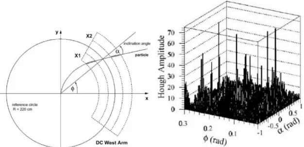
5.1 Left:The definition α and ϕ. Right: An example scatter distribution of α and ϕ of all possible pairs. . . 55

5.2 Centrality classes in the EZDC vs. charge in BBC scatter plot. . . 55

5.3 Left:The distribution of the distance between the best quality tracks at PC1 in typical MB run in 0∼800 cm. Right:The distribution of the distance between the best quality tracks at PC1 in typical MB run in 0∼18 cm. . . 57

5.4 Left:The distribution of the distance between the best quality tracks at PC1 in typical UPC run in 0∼800 cm. Right:The distribution of the distance between the best quality tracks at PC1 in typical UPC run in 0∼18 cm. . . 57

5.5 Momentum interpolation grid. . . 58

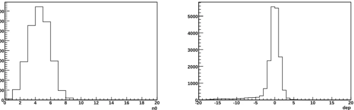
5.6 Left: The simulated n0 distribution of electrons. Right: The simulated dep distributions of electrons. . . 59

5.7 The simulated √ (emcsdphie× emcsdphie+ emcsdze× emcsdze) distribution of electrons. . . 59

5.8 The distribution of zBBC − zP C1track . . . . 60

5.9 Left:The distribution of electrons (left) ϕdc (zed) and zedpc(cm) of reference run. The distribution of positrons ϕdc (zed) and zedpc (cm) of reference run [63] . . . 61

(11)

5.10 Upper left: The scatter distribution of the electron multiplicity of ysect and

zsect at sector 2, where ysect and zsect means EMCal tile id. Upper right:The

scatter distribution of the ratio of total per electron (Rel/tr) of ysect and zsect at

sector 2. Lower left: The distribution of the Rel/tr of overall towers at sector 2.

Lower right:The scatter distribution of the excluded sectors of ysect and zsect

at sector 2. [63] . . . 62

5.11 The scatter distribution of ϕrich(zed) and zedrich(cm) of reference run[63] . . . . 63

5.12 The scatter distribution of zBBC and _tan(θ)1 of reference run[63] . . . 64

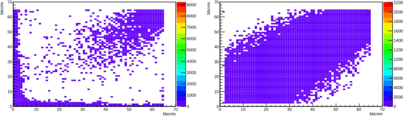
5.13 Left:The distributions of NBBCN and NBBCS of the UPC sampled events. Right:The

distributions of NBBCN and NBBCS of the MB sampled events. . . 66

5.14 The Ntrack distributions, UPC(red), MB with ERT2x2(blue), and UPC with

NBBCN = 0&NBBCS = 0 (magenta) are compared. To use a same vertex range,

|zZDC| <30 cm are required for all distributions. The MB distribution is

nor-malized to the UPC distribution from 40 to 100. . . 66

5.15 The distribution of electron pair mass of all data which was taken by UPC trigger

in the 2007 PHENIX run without any cut . . . 68

5.16 Left:Ntrack distribution where the events have the pairs with mass from 0.5 to

2.0 GeV. Right:Ntrack distribution where the events have the pairs with mass

from 2.0 GeV. Red (blue) line corresponds to unlike (like) sign pair. . . 68

5.17 Left:Ntrackdistribution with ”(EZDCN > 30 GeV| EZDCS > 30 GeV)&|zP C| <30

cm & (NBBCN =0|NBBCS =0)” where the events have the pairs with mass from

0.5 to 2.0 GeV . Right:Ntrack distribution with ”(EZDCN > 30 GeV | EZDCS >

30 GeV)& |zP C| <30 cm & (NBBCN =0|NBBCS =0).” where the events have the

pairs with mass from 2.0 GeV. Red (blue) line corresponds to unlike (like) sign

pair. . . 69

5.18 Left:The distributions of electron pair mass with ”(EZDCN > 30 GeV| EZDCS >

30 GeV)& |zP C| <30 cm & (NBBCN =0|NBBCS =0) & Ntrack =2”. The red

(blue) line corresponds to unlike (like) sign pair. Right: The distributions of

electron pair mass and pair pT with ”(EZDCN > 30 GeV | EZDCS > 30 GeV)&

|zP C| <30 cm & (NBBCN =0|NBBCS =0) & Ntrack =2”. . . 70

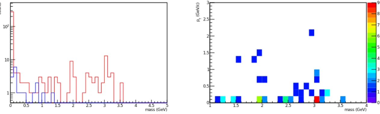
5.19 Left:The distributions of electron pair mass. Right:Its Ntrack distribution where

the events have the pairs with mass from 2.7 to 3.5 GeV. The red (blue) line

corresponds to unlike (like) sign pairs. . . 71

5.20 A comparison plot of unlike-sign Ntrack distributions of 2007 UPC and 2006 p+p. 72

5.21 The distributions of NBBCN and NBBCS for diﬀractive process. Simulated by

PYTHIA. . . 73

5.22 Left: The distribution of the number of electrons (positrons), Simulated by

PYTHIA. Right: The distribution of the npart muon for diﬀrative process. . . 74

5.23 The simulated data invariant mass of unsign pairs (blue-colored) and

like-sign pairs (red-colored) for Nelectron/positron == 2 (left plot). dN/dpT

distribu-tion in [2.0,4.0] (right plot). . . 75

5.24 The scatter plot ofϵERT 2x2and mee, and its fitting result with ϵcontinuumERT 2x2 (me+_e−) =

a× (me+_e−− b)2+ c. The left panel is for before run 235000, and the right is for

(12)

5.25 Left:The MB (BLUE), ERT2x2 (RED) and subtracted ERT2x2 (magenta)

trig-gered cluster dN/dpT distributions at sector0 in run231155. Right: ERT2x2 turn

on curve at sector0 in run231155. . . 78

5.26 Left:pT > 2GeV hit map with only fiducial cut in [63] at run231155 sector0. Right:pT > 2GeV hit map with new noisy list at run231155 sector0. . . . 78

5.27 Thep0 values for each sector and run. . . 80

5.28 The p1 values for each sector and run. . . 80

5.29 The p2 values for each sector and run. . . 80

5.30 Left: The simulated full transversely polarized case invariant mass distributions and the single-Gaussian fitting results. Right: The simulated unpolarized case invariant mass distributions and the single-Gaussian fitting results. . . 84

5.31 The simulated invariant mass distribution and the double-Gaussian fitting re-sults. The left panel is the full transversely polarized case and the right one is the unpolarized case. . . 84

5.32 The simulated reconstructed pT distributions of e+e− pairs from J/ψ with gen-erated pT , 0.0∼0.01, 0.5∼0.51 (Red), 1.0∼1.01 (blue), and 2.0∼2.01, GeV/c . . 84

5.33 The black crosses correspond to (1/2πpT)d2N /dpTdy [(GeV/c)−2]of J/ψ in p+p collisions [70]. Fitting function is p0(1 + pT/p1)−6 . . . 85

5.34 The pT dependence of simulated Acc × eﬃciency of transverse polarized (Red line) and unpolarized (Black line) case. The blue line is the actually used Acc × eﬃciency. . . . 86

5.35 Left:The pT dependence of ϵERT 2x2ef f ectivefor transverse polarized J/ψ at before run23500. Right:The pT dependence of ϵERT 2x2ef f ectivefor transverse polarized J/ψ at after run23500. Please note scatter plot was not weighted because of to help seeing. . . 86

5.36 Left:The pT dependence of ϵERT 2x2ef f ective for unpolarized J/ψ at before run23500. Right:The pT dependence of ϵERT 2x2ef f ective for unpolarized J/ψ at after run23500. . . 87

5.37 Left:The real data dN/dmee plots. The fitting function is shown as the black line. The blue line is continuum e+e− part. The red line is J/ψ part. Right:The pT distribution within J/ψ area (3 σ). . . . 88

5.38 The continuum pair pT distribution within 3.096 ± 3 × 0.074 GeV/c2 using starlight model [40] . . . 89

5.39 The subtracted pair pT distribution. . . 89

5.40 Left :The 300 times random fitting results. Right:corresponded number of J/ψ dis-tribution. . . 90

5.41 The (1/2πpT)d2N /dpTdy [(GeV/c)−2]distribution in Ultra-Peripheral Au-Au Col-lisions at √sN N = 200 GeV in the 2007 run. . . 92

5.42 The measured cross-section compared to theoretical [40, 38, 41, 42, 42, 43] and the 2004 result. . . 93

5.43 2004 and 2007 combine cross-section compared to theoretical [40, 38, 41, 42, 42, 43]. . . 94

5.44 Left:The real data dN/dmee plots with +XnY n condition. The fitting function is shown as the black line. The blue line is continuum e+e− part. The red line is J/ψ part. Right:The pT distribution within J/ψ 3 σ . . . 95

(13)

6.2 The distribution of x and y position of muon tracks in UPC real data files in the

South arm. Left:when oct4 has a big hole. Right:oct8 has a big hole. . . 100

6.3 Left:The invariant-mass distributions of the µ+µ−pairs with the non-multiplicity

cut, ”|zzdc| <30 cm& (EZDCN > 30GeV & EZDCS > 30 GeV & (NBBCN=0|NBBCS=0)”

in North arm. Right:The invariant-mass distributions of the µ+µ− pairs with the

non-multiplicity cut, ”|zzdc| <30 cm& (EZDCN > 30GeV & EZDCS > 30 GeV &

(NBBCN=0|NBBCS=0)” in South arm. . . 101

6.4 Left:The distributions of Ntrack for µ pair in the North arm where the events

have the pairs with mass from 2.7 to 3.5 GeV with the non-multiplicity cut.

Right:The distributions of Ntrack for µ pair in the South arm where the events

have the pairs with mass from 2.7 to 3.5 GeV with the non-multiplicity cut. The

red (blue) line corresponds to unlike (like) sign pair. . . 102

6.5 The distributions of RXNP charge with the cut of ”|zzdc| <30 cm& (EZDCN >

30GeV & EZDCS > 30 GeV)& (NBBCN=0|NBBCS=0)&(2.7< mass <3.5 GeV)

”. Upper (Under) two figures correspond to when dimuon pair is detected by the north (south) arm. The charge of the north (south) RXNP is shown in Left

(Right) panel. . . 102

6.6 Same as Fig 6.5, with adiﬀerent x-axis scale, in order to see. . . 103

6.7 The distributions of Ntracks at 2.6∼3.6 GeV/c2 with the cut of ”|zzdc| <30 cm&

(EZDCN > 30GeV & EZDCS > 30 GeV )& (NBBCN=0|NBBCS=0)& (Qrxnpn<1000

& Qrxnps¡1000)&(2.7< mass <3.5 GeV)”. . . . 103

6.8 Left:The distributions of muon pair mass for the final sample in North arm. The

red (blue) line corresponds to unlike (like) sign pair. Right: The correspond

—PT distribution. . . 104

6.9 Left:The distributions of muon pair mass for the final sample in South arm. The

red (blue) line corresponds to unlike (like) sign pair. Right: The correspond

—PT distribution. . . 104

6.10 The ZDC energy deposit distributions of the final samples at 2.6 3.6 GeV/c2 .

Left (Right) two panels correspond to the north (south) ZDC. Upper (Lower)figures

corresponds to when dimuon is detected by the north (south ) arms. . . 105

6.11 Left:The dimuon invariant mass yields of p+p collisions at √s= 200 GeV in

2009 year in the North arm. Right:The dimuon invariant mass yields of p+p

collisions at √s= 200 GeV in 2009 year in the South arm. The red (blue) lines

corresponds to unlike (like) sign pair. . . 106

6.12 The distributions of Ntrack for µ+µ− pairs where the events have the pairs with

mass from 2.6 to 3.6 GeV. p+p collisions at√s= 200 GeV in the 2009 PHENIX

run. . . 107

6.13 Left:The dimuon invariant mass yields of p+p collisions at √s= 200 GeV in the

2009 PHENIX run in the North arm with Ntrack=0. Right:The dimuon invariant

mass yields of p+p collisions at √s= 200 GeV in the 2009 PHENIX run in the

South arm with Ntrack=0. The red (blue) line corresponds to unlike (like) sign

(14)

6.14 Left:The normalized distributions of mass for µ+µ− pair where the events have

the pairs with mass from 2.6 to 3.6 GeV in p+p collisions at √s= 200 GeV

in the 2009 PHENIX run in the North arm to have 2.8 J/ψ events. Right:The

normalized distributions of mass for µ+µ− pair where the events have the pairs

with mass from 2.6 to 3.6 GeV in p+p collisions at √s= 200 GeV in the 2009

PHENIX run in the South arm to have 2.8 J/ψ events. The red (blue) line corresponds to unlike (like) sign pair. The left (right) side corresponds to the

north (south). . . 108

6.15 Normalized pT distribution where the events have the pair with mass from 2.6

to 3.6 GeV/c2 _{in p+p collisions at} √_{s= 200 GeV in the 2009 PHENIX run.} _{. . 108}

6.16 Left:The generated rapidity distribution of γγ →µ+µ− where the events have

the pairs with mass from 2.0 to 4.0 GeV and 5 > |y| using starlight model.

Right :That of invariant mass. . . 109

6.17 Left:The simulated distribution of detector passed invariant mass in the North arm. Right:The simulated distribution of detector passed invariant mass in the South arm. The red lines show all generated and the blue line is normalized to luminosity in the 2010 PHENIX run. . . 109

6.18 Left:The simulated distribution of detector passed pT in the North arm. Right:The

simulated distribution of detector passed pT in the South arm. . . 110

6.19 Left:The fitted invariant mass distribution and fitting result in the North arm

of p+p collisions at √s= 200 GeV, pT <0.5 GeV/c . Right:The fitting result

in the North arm of UPC at √s= 200 GeV, pT <0.5 GeV/c . The red (blue)

crosses correspond to unlike (like) sign pair and the black crosses correspond to subtracted. The black line corresponds to the fitting result, light blue line

corresponds to continuum background . . . 111

of p+p collisions at √s= 200 GeV, 0.5 < pT <1.0 GeV/c . Right:The fitting

result in the North arm of UPC at √s= 200 GeV, 0.5 < pT <1.0 GeV/c . The

red (blue) crosses correspond to unlike (like) sign pair and the black crosses correspond to subtracted. The black line corresponds to the fitting result, light

blue line corresponds to continuum background . . . 112

6.21 Left:The fitted invariant mass distribution and fitting result in the North arm of

p+p collisions at√s= 200 GeV, 1.0<pT <1.5 GeV/c . Right:The fitting result in

the North arm of UPC at √s= 200 GeV, 1.0<pT <1.5 GeV/c . The red (blue)

(15)

6.23 Left:The fitted invariant mass distribution and fitting result in the North arm of

the North arm of UPC at √s= 200 GeV, 2.0<pT <2.5 GeV/c . The red (blue)

6.27 Left:The fitted invariant mass distribution and fitting result in the South arm

of p+p collisions at √s= 200 GeV, pT <0.5 GeV/c . Right:The fitting result

in the South arm of UPC at √s= 200 GeV, pT <0.5 GeV/c . The red (blue)

result in the South arm of UPC at √s= 200 GeV, 0.5 < pT <1.0 GeV/c . The

6.29 Left:The fitted invariant mass distribution and fitting result in the South arm of

the South arm of UPC at √s= 200 GeV, 1.0<pT <1.5 GeV/c . The red (blue)

(16)

result in the South arm of UPC at √s= 200 GeV, 1.5 < pT <2.0 GeV/c . The

6.31 Left:The fitted invariant mass distribution and fitting result in the South arm of

the South arm of UPC at √s= 200 GeV, 2.0<pT <2.5 GeV/c . The red (blue)

6.32 Left:Scatter distribution xpos1 and ypos1 of simulated muon tracks in the North

arm. Right:Same one in the South arm. . . 121

6.33 Left:Scatter distribution xpos2 and ypos2 of simulated muon tracks in the North

6.34 Left:Scatter distribution xpos3 and ypos3 of simulated muon tracks in North

6.35 Left:Scatter distribution xpos4 and ypos4 of simulated muon tracks in North

6.36 Left:The simulated measured mass distributions of J/ψ pairs with generated pT,

0.0∼0.01, 0.5∼0.51 (Red), 1.0∼1.01 (blue), 3.0∼3.01 (magenta), and 5.0∼5.01(green) GeV/c in North arm. Right:Same one in the South arm. . . 123

6.37 Left:The simulated measured pT distributions of J/ψ pairs with generated pT,

0.0∼0.01, 0.5∼0.51 (Red), 1.0∼1.01 (blue), 3.0∼3.01 (magenta), and 5.0∼5.01(green) GeV/c in North arm. Right:Same one in the South arm. . . 123

6.38 Left:The real−dN/dpT

Acc×ϵ distributions and its fitting result. Right:The

real−dN/dy Acc×ϵ

distributions and its fitting result. In each figure, Black line corresponds to unpolarized pairs in the North arm, red corresponds to full transverse polarized pairs in the North arm, blue corresponds to unpolarized pairs in the South arm,

magenta corresponds to full-polarized pairs in the South arm. . . 124

6.39 Left: The real−dN/dpT

Acc×ϵ distributions and their fitting results. Right:The

real−dN/dy Acc×ϵ

distributions and their fitting results. In each figure, Black line corresponds to unpolarized pairs in the North arm, red corresponds to full transverse polarized pairs in the North arm, blue corresponds to unpolarized pairs in the South,

magenta corresponds to full-polarized pairs in the South arm. . . 125

6.40 Left:The rapidity integrated pT dependence of (Acc· ϵreco · ϵcuts) in the North

arm. Right:The rapidity integrated pT dependence of (Acc· ϵreco· ϵcuts) in the

South arm. . . 126

6.41 The pT integrated rapidity dependence of (Acc· ϵreco· ϵcuts). . . 126

6.42 The pT distributions of UPC J/ψ The red (blue) line corresponds to north

(17)

6.43 Left:The rapidity distribution of p+p unlike-sign pairs where the event has the

pair with mass form 2.6 to 3.6 GeV/c2 _{. Right:The rapidity distribution of final}

samples where the event has a pair with 2.6GeV/c2 ≤ mass. Both distributions

are normalized to expected yield . . . 128

6.44 Left:The rapidity distribution UPC J/ψ. Right:rapidity distribution of final

samples at 2.6 ∼ 3.6 GeV/c2 _{(without subtraction).} _{. . . 128}

6.45 The d2σ/dpTdy distribution of UPC J/ψ +XnY n in the 2010 PHENIX run. The

blue line corresponds to the result of the South arm, the red line corresponds to the result of the North arm. The magenta line corresponds to result of the

central arm. . . 130

6.46 The dσ/dy distribution of both side neutron tagged J/ψ → µ+_µ−_{in the 2010}

PHENIX run. . . 131

7.1 Right : The 2004 and 2007 combined cross-section compared to theoretical

curves [30, 40, 38, 41, 42, 43]. Left :The 2004 and 2007 combined cross-section compared to theoretical curves [38, 41] of coherent + incoherent . . . 134

7.2 Left: dσ/dy compared to theoretical curves [30, 40, 38, 41, 42, 43] of coherent or

incoherent and the previous result in the 2004 PHENIX run. Right: dσ/dy com-pared to theoretical curves [38, 41] of coherent + incoherent and the previous

result in the 2004 PHENIX run. . . 134

7.3 The (1/2πpT)d2N /dpTdy [(GeV/c)−2]distribution in Ultra-Peripheral Au+Au

Collisions at √sN N = 200 GeV in the 2007 PHENIX run. . . 135

7.4 _dydpd2σ

T of UPC J/ψ +XnY n in Au+Au at

√

sN N = 200 GeV in the 2010 PHENIX

run. . . 137

(18)

(19)

List of Tables

3.1 The Basic spec of RHIC at heavy ion runs. . . 19

3.2 Parameters of PCs . . . 33

3.3 The azimuthal oﬀset angles between wires of stereo and non stereo planes. . . . 40

4.1 Triggers and typical rate in 2007 PHENIX run . . . 48

4.2 Triggers and typical rate in 2010 PHENIX run . . . 48

5.1 The definition of reconstructed track. . . 56

5.2 Cut and events . . . 65

5.3 bbc . . . 76

5.4 The noisy tower list . . . 79

5.5 The projection result of Fig 5.27 5.28 5.29. . . 81

5.6 The count in each pT bins of the original, normalized continuum e+e−,and sub-tracted. . . 90

5.7 The (1/2πp_√ T)d2N /dpTdy [(GeV/c)−2]in Ultra-Peripheral Au-Au Collisions at sN N = 200 GeV in the 2007 run. . . 92

6.1 bbc . . . 118

6.2 bbc . . . 119

6.3 The A and B values of each iteration step in unpolarized case . . . 125

6.4 The A and B values of each iteration step for full pol case . . . 125

6.5 The extraction of dNJ/ψ/dpT distribution of UPC J/ψ +XnY n in the 2010 PHENIX run . . . 127

6.6 The extraction of dNJ/ψ/dyof both side neutron tagged J/ψ→ µ+µ−in the 2010 PHENIX run . . . 129

6.7 The d2_σ/dp Tdy of UPC J/ψ +XnY n in the 2010 PHENIX run . . . 130

(20)

(21)

Chapter 1 Introduction

In 1969, in the ep deep inelastic scattering (DIS) experiment at Stanford Linear Accelerator Center (SLAC) found point like particles were found inside the nucleon [1]. Since then, there have been many experiments to study the inner structure of the nucleon at CERN, DESY, and FNAL [2]. These experiments showed a nucleon is a complex object with valence quarks, sea quarks and gluons.

The momentum distribution of partons inside a nucleon, called as a Parton Distribution

Function (PDF), has been measured as a function of Bjorken x and Q2 _{being the energy scale}

of the hard interaction.

Especially, HERA found a rapid increase of the gluon distribution with decrease x are

shown in Fig 1.1 [1].

In the lA experiments, notable nuclear modification of PDF was found [3, 4, 5, 6, 7, 8, 9, 10]. However, its mechanism and amplitude are not well understood theoretically. Recently, ultra-peripheral heavy ion collisions have attracted great interests to study the parton distribution in the nucleus by using the strong electromagnetic fields that act as a field of photons provided by fast moving heavy ions. Especially, exclusive photo-nuclear vector meson production is a sensitive probe of gluons inside nuclei. Ultra-peripheral collision (UPC) is the collision whose impact parameter is larger than the sum of the two nuclear radii. The γ flux of the UPC is

proportional of the square charge of the nuclei, Z2_.

In this thesis, J/ψ productions in the UPC are studied at Au+Au collisions at RHIC-PHENIX in Brookheaven National Laboratory. The maximum center of mass energy in the

γAu system is 34 GeV, which is large enough to produce a J/ψ. The UPC J/ψ measurement

at RHIC is sensitive to the gluon distributions in the nucleus down to x∼= 0.015, at Q2 =2.5

(GeV/c)2_.

The PHENIX already published the measurement of J/ψ production in ultra-peripheral collisions using the data samples taken in 2004 [30]. Only the total cross section at the central rapidity was measured, and it has too low statics to discuss non-linear Quantum

chromodynam-ics (QCD) evolution at small x. The purpose of this study is to measure the pT dependence of

the cross section by using data which was taken in 2007. The cross section of J/ψ production in the UPC (UPC J/ψ ) is a relatively simple process so that is useful to study low x QCD.

The PHENIX detector has wide acceptance in both central and forward rapidity regions.

The cross sections and its pT dependence of UPC J/ψ in the forward rapidity region are

(22)

Figure 1.1: Gluon, sea and u and d valence distributions extracted by HERA-ZEUS at

(23)

The organization of the thesis is as follows. A brief summary of related theoretical back-ground is described in Chapter 2. The experimental setup, the RHIC accelerator and PHENIX detectors are briefly explained in Chapter 3. The detail of trigger and conditions in 2007

and 2010 PHENIX runs are described in Chapter 4. The detail of analysis of 2007 UPC

J/ψ → e+_e− _{at central rapidity and 2010 UPC J/ψ}_{→ µ}+_µ− _{at forward rapidity are presented}

in Chapter 5 and 6, respectively. The results and discussions are shown in Chapter 7. The summary is given in Chapter 7.

Major Contribution

The author carried out the measurement and analysis of J/ψ photo-production with J/ψ →

e+_e− _{and J/ψ} _{→ µ}+_µ− _{channels for the 2007 and 2010 runs at the PHENIX experiments. The}

author took the responsibilities of the operation and calibration of the Ring Imaging Cherenkov Counters.

(24)

(25)

Chapter 2 Theoretical backgrounds

2.1 Deep inelastic scattering and nucleon structure

In the inclusive measurements of the deep inelastic scattering, kinematics can be described by

two variables. An example choice is the negative square of momentum transfer, Q2 and the

Bjorken x which is defined as Q2_{/2M ν, where M is mass of the target and ν is the energy}

transfer between incoming and outgoing lepton at the rest frame of the target.

2.1.1 Kinematics of deep Inelastic collisions and PDF

Start from the simplest case. The diﬀerential cross section of A+B is described by the following equation. dσ dΩ = α2cos2 θ₂ 4E2_sin2 θ 2 ( ≡ dσ dΩM ott ) , (2.1)

where m is the mass of A and M is the mass of B, α is the electromagnetic coupling constant,

θ is the scattering angle, and E is the incident energy. m/M ≪1 is assumed. If the probe (A)

and target (B) have spin 1/2, the diﬀerential cross section in fixed target A+B elastic scattering is described by the following equation.

dσ dΩ = dσ dΩM ott E′ E [ 1− q 2 2M2 tan 2 θ 2 ] , (2.2)

where E and E′ are initial and final energy of A, and q is the momentum transfer. If B is not

point like particle, a form factor (F ) is introduced. It is Fourier transformation of the density

function (ρ(⃗r)) defined as,

F (q2) = ∫

(26)

The elastic cross section is then described in the form of dσ dΩ = dσ dΩM ott E′ E [( F₁2+ κ 2_Q2_F2 2 4M2 ) − (F1+ κF22) 2 Q2 2M2tan 2 θ 2 ] , (2.4)

where F1 and F2 are form factors, F1(0) = 1, F2(0) = 1, and κ is the anomalous magnetic

moment .

For the inelastic scattering, which includes all possible final states, the inclusive scattering

cross section is expressed as follows with an extra variable, the final A energy (E′)

d2_σ dΩdE′ = dσ dΩM ott [ W2(Q2, ν) + 2W1(Q2, ν) tan2 θ 2 ] , (2.5)

where ν = E − E′ and W1, W2 are structure functions which are related to ρ. Once, d

2_σ

dΩdE′ is

measured in a many Q2 , ν points, ρ(⃗r) is deduced. The formula can be converted to x and y

variables (Bjorken x and rapidity y ≡ nu/E).

d2_σ dxdy = 4πα2_s Q4 [ 2xF1 1 + (1− y)2 2 + (1− y)(F2− 2xF1)− M 2ExyF2 ] , (2.6)

where s is the square of the center-of-mass energy and 2M E. F1 and F2 are diﬀerent form

factors from the ones in Eq. 2.4. This new structure functions are related to W1,2 such as

F1 = M W1 and F2 = νW2.

2.1.2 Parton model

At the beginning of DIS experiments, the region of x∼0.1 was covered in the measurements.

As shown in Fig 2.1, F2 is independent of Q2 in the region (Bjorken scaling).

To reproduce the scaling, parton model is proposed. The basic ideas of parton model are following;

• Nucleon is consistent of point like particles (parton).

• At the time of the interaction, they can be seen as a collection of free particle . • However, they are bound in the nucleon.

In this picture, dσ/dy of virtual photon and ith parton is as follows,

dσ dy = 4πα2_xs Q4 [ 1 + (1− y)2 2 − M 2E ] λ2_iqi(x)dx, (2.7)

where qi(x) and λi are momentum distribution function and charge of ith parton, respectively.

Therefore, dσ/dy of virtual photon and proton is

d2σ dxdy = 4πα2xs Q4 [ 1 + (1− y)2 2 − M 2E ] Σλ2_iqi(x)dx. (2.8)

(27)

(28)

To compare with Eq. 2.6

F2 = 2xλ2iqi(x) (2.9)

F1 = F2/2x (2.10)

The equations show dimensionless structure functions are independent of Q. In this picture,

F2 is the charge-square weighted distribution of partons. Through the measurement of

struc-ture functions, momentum distribution of the parton can be deduced. x corresponds to the momentum fraction of the proton carried by the parton in the picture.

As shown in Fig 2.1, in recent years, in the lower x regions, F2 was found to depend on Q2 .

As diﬀerent from parton model, interaction between partons plays an important role, therefore

Q2 _{independence is disturbed. In the region of x}∼0.1, Q2 _{independence is incidentally}

consistent.

2.1.3 DGLAP equation

Dokshitzer-Gribov-Lipatov-Altarelli-Parisis (DGLAP) equations describe the Q2 _dependence

of PDF based on the QCD [11].

From the equations, the distributions for the higher Q2 _{are predicted. At the limit of high}

Q2 _{where the transverse momentum of the partons are neglected, the evolution of the quark}

(q) and gluon (g) distribution functions can be written as;

dq(x, Q2) d ln Q = αs(Q2) π ∫ ₁ x dξ ξ Pq←q(ξ)q(x/ξ, Q) + Pq←gg(x/ξ, Q), (2.11) dg(x, Q2) d ln Q = αs(Q2) π ∫ ₁ x Pg←q(ξ)Σi[qi(x/ξ, Q) +qi(x/ξ, Q)] + P¯ g←gg(x/ξ, Q), (2.12)

(29)

2.2 Parton distribution function in nuclei

It has been known that the structure function in the nucleus (AFA

2 ) is not identical to that in

free nucleons (F₂p) from several experiments [5], as shown in Fig 2.2. The dominant Nuclear

Figure 2.2: The ratio of F2structure functions of various nuclei to that of deuterium [5]

eﬀects each x region are as follows.

• x∼ 1: Fermi motion enhances scattering around the limit.

• 0.3≤ x ≤ 1:The decrease is at first discovered by the EMC exp, and hence called EMC

eﬀect. The origin is still discussed.

• 0.03≤ x ≤ 0.3:The enhancement in this region is often referred as anti-shadowing. The

(30)

• x≤ 0.03:At low-x RAagain become less than 1. The origin is still discussed.

One convention to relate the PDF of nucleon and nuclei is to introduce the nuclear modifi-cation factor (R), defined as

q_iA(x, Q2) = ARA_i (x, Q2)q_ip(x, Q2), (2.13)

where qi is the PDF of the ith species of quarks or g for gluons. Any deviation from R = 1 is

regarded as nuclear eﬀects.

As seen in Fig. 2.2, shadowing of F2 is experimentally well established. However, there are

no well accepted background theory. Since gluon has no charge so that can’t be probed directly via DIS or DY at lowest order, gluon PDF of the nuclei remains largely unknown.

Various theoretical models of RF2 and Rg are shown in Fig. 2.3. They are based on DIS

and DY experiments and DGLAP equation. At x∼0.01, RF2s have almost same values, on the

other hand, Rgs have a wider range.

Figure 2.3: Left:F2 ratios for Pb versus x at fixed Q2= 3 GeV2from various models [12,

13, 14, 15, 16, 17, 18, 19, 20, 21]. Ratios of gluon distribution functions for Pb versus x from

diﬀerent models at Q2 = 5 GeV2 [12, 13, 14, 15, 16, 17, 18, 19, 20, 21]

Poor understanding of Rgis due to the lack of the gluon sensitive measurements. In Fig. 2.3,

only the middle point of various theoretical predictions are shown. For example, theoretical

(31)

(32)

2.3 J/ψ production in ultra-peripheral collisions

To study parton distribution function of nuclei, photo-production process with ultra-peripheral collision (UPC) has attracted great interests for recent years. [23, 24, 25]. Ultra-peripheral means that the impact parameter of the collision is larger than twice the nucleus radius so that the two nuclei do not overlap with each other. A relativistically moving ion emits a quasi real

photon with maximum energy ∼ γ/R, where γ is γ factor of the nuclei and R is the radius

[26, 27]. At RHIC, the maximum energy of heavy ions with √sN N = 200 GeV, energy of quasi

real photons can reach about 3 GeV and the center of mass energy of γA system can be √sγA=

34 GeV.

2.3.1 Cross section estimation in p+p collisions

The lowest order diagram of J/ψ photo-production in Au+Au collisions is shown in Fig. 2.5. The two-gluon picture is applicable to the production of heavy vector mesons. On the simplest

Figure 2.5: The diagram of J/ψ production.

assumption, and in the simplest p+p or e+p collisions, the production cross section is expressed as follows. dσ dt(γ ∗_p_{→ J/ψp)|} 0 = ΓeeMJ/ψ3 π w 48α αs( ¯Q2)2 ¯ Q8 [xg(x, ¯Q 2_)]2_{(1 +} Q2 M2 J/ψ ), (2.14)

(33)

where Γee is the electronic width of the J/ψ , MJ/ψ is the rest mass of J/ψ , ¯Q = (Q2 +

M2

J/ψ)/4, and x = 4 ¯Q2/W2 [28]. Therefore, the photo-production cross section is proportional

to the square of gluon density. It shows that the cross section can be a sensitive to the gluon PDF of nuclei.

2.3.2 Cross section estimation in A+A collisions

To estimate UPC J/ψ cross section in A+A collisions, there are two major approaches.

Collinear approach

Collinear approach is based on Eq. 2.14 and nuclear PDF (nPDF). The nPDF is RA modified

PDF. Some of theorists estimate cross section of UPC J/ψ +Xn (with neutron emission) in RHIC with this approach [29]. The detail of neutron tagging is discussed later. The theorist used the nuclear breakup probability, 0.64 (64% of UPC J/ψ events are associated with at least a neutron). This is higher than that of the assumed values in the PHENIX previous measurement, 0.55 [30, 31]

Figure 2.6: Left:Theoretical prediction of R_Aug . Right:2004 UPC J/ψ +XN result with theoretical predictions [30, 29, 32, 33, 34, 22].

Color dipole approach

The basic idea of this approach is that photons can take vector meson state, virtually [35]. In the target frame, γA scattering can be taken as vector meson + nuclei collisions.

In the framework, lifetime of virtual photon in VM state:

∆t = 1/∆E, ∆E = EV M − Eγ∗ = √ M2 V M + p2γ− √ q2_{+ p}2 γ ∼ M2 V M + Q2 2pγ (2.15)

(34)

mo-mentum of virtual photons. Then,

c∆∼ 2pγ

M2

V M + Q2

>> RA (2.16)

Vector meson states live long enough to interact several times in the nucleus. The leading twist (LT) order contribution is taken as an origin of the shadowing in the theorem. The diagram of LT contribution and γp diﬀractive process are shown in Fig. 2.7 [36, 37]. These diagrams are closely related. Therefore, shadowing eﬀect is related to the J/ψ and nuclei cross section,

σJ/ψN, and it can be estimated diﬀractive PDF from HERA data.

Figure 2.7: The diagram of LT contribution and γp diﬀractive process [36].

In both approaches, UPC J/ψ cross section reflects gluon dynamics in nuclei, therefore the measurement plays important role to study low x QCD.

2.3.3 Physical processes in UPC at RHIC energy

In the RHIC energy region, the following three processes are expected to be competitive in the UPC.

• Coherent J/ψ production (γAu →J/ψ +Au): The _dpdσ

T distribution will have a very

narrow peak at t ≤0.015 GeV2_{, because higher momentum transfer is suppressed due to}

the nuclear form factor.

• Incoherent J/ψ production (γN →J/ψ +Au∗): The collision is assumed as γ and one

of nucleon in the nuclei collision. The _dpdσ

T distribution will have a wider shape than the

(35)

• In addition, as a background , a lepton pair is produced via a two photon process (γγ→

ll):Especially, in the mid-rapidity region, γγ →e+_e− _{can be the main background source.}

Forward neutron emission

The photons to the right of the dashed line are soft photons that may excite the nuclei in Fig. 2.5. A Coulomb excitation leads to emission of neutrons in the very forward direction. PHENIX can make triggers only for UPC J/ψ events with neutrons +Xn (detail is discussed in the Chap. 4).

In coherent UPC case, J/ψ production and neutron emission are independent. It means that neutron tagging does not introduce any biases in the extraction of exclusive J/ψ cross section

from these events. On the other hand, in incoherent case (γN →J/ψ +Au∗), the nucleon

will be recoiled. The recoiled nucleon with the residual nucleus react and emit neutrons,

N + (A− 1) = Ci+ kn [38].

Figure 2.8: Left:Theoretical prediction of Integrated over rapidity (|y| < 3) the

momen-tum transfer distributions for the J/ψ in the coherent (solid line) and incoherent (dashed line) photoproduction in UPC of Au ions at RHIC [38]. Right:Theoretical prediction of incoherent UPC J/ψ number of emitted neutron distribution without any trigger

require-ment at√sN N = 200 GeV [38].

In this analysis in forward rapidity, both side neutron tagging is required (detail is discussed in Chap. 6). Only Strikman [39] made a prediction for XnY n tagging UPC J/ψ at RHIC. Figure 2.9 shows the prediction.

(36)

Figure 2.9: Theoretical prediction of UPC J/ψ cross section distribution with any trigger

requirement at √sN N = 200 GeV. Black dots are old preliminary result, they can be

(37)

2.3.4 Previous PHENIX UPC J/ψ result and predictions

PHENIX already published combined dσ_dy of J/ψ +Xn at |η| < 0.35 with the data taken in

2004 [30] with Lint= 121 µb−1. Clear J/ψ peak can be seen, and the number of J/ψ is 9.0±

4.0 ± 1.0. As shown in Fig 2.10, the result is consistent with many predictions within its statistical error. Since there is low statistics, the previous result is coherent and incoherent

Figure 2.10: Left:dN/dmee distribution fitted to the combination of a dielectron

con-tinuum (exponential distribution) and a J/ψ (Gaussian) signal at √sN N =200 GeV in

the 2004 PHENIX run [30]. Right:2004 UPC J/ψ +XN result with theoretical predic-tions [30, 40, 38, 41, 42, 43].

combined result. Following thoretical models are presented in Fig 2.10. • starlight : Just for comparison, parameterize to HERA data [40].

• Strikman: Leading twist order shadowing, σJ/ψN is assumed to 3 mb [38].

• Kopeliovich:Leading twist order shadowing, the dipole cross section is treated as a

func-tion of rt,

√

s, where√s is the center of mass energy, and rT is the transverse q ¯q separation.

Calculations were performed with KST and GBW parameterizations for the dipole cross section, [41].

• Goncalves-Machado: Gluon saturation is assumed [42].

In the figure, based on starlight [31], theoretical curves are modified with the nuclear breakup probability, 0.55.

(38)

(39)

Chapter 3 Experimental setup

Experimental set up of RHIC PHENIX are presented in the chapter.

3.1 Relativistic Heavy Ion Collider (RHIC)

The RHIC is the first heavy ion collider in the world. The basic parameters of RHIC in heavy ion runs are shown in Fig. 3.1.

Its maximum center of mass energy per nucleon pair is √sN N = 200 GeV. It can also be

operated with proton-proton collision mode with √s up to 500 GeV It started its operations

in 2000 [44].

The schematics of the RHIC accelerator complex are shown in Fig. 3.1. The RHIC ac-celerator complex is composed of a Tandem Van de Graﬀ, the proton linac, the booster syn-chrotron, the Alternating Gradient Synchrotron (AGS), and the RHIC rings. STAR [45] and PHENIX [46] are the main experiments at RHIC and two small experiments (BRAMHS [47] and PHOBOS [48]) were conducted until 2012.

Table 3.1: The Basic spec of RHIC at heavy ion runs.

Injection Energy γ =10.25 (p = 9.5 GeV/c /nucleon)

Storage Energy γ= 107.4 (p = 100.0 GeV/c /nucleon)

Peak Luminosity 30×1026 cm−2/s

Ions/Bunch 1.1×109

Number of bunches 111

Emittance 17−35 µm

Interaction diamond length (maximum) 20 cm

Crossing angle, nominal (maximum) 0(<1.7) mrad

Bunch length 15 cm

Bunch radius 0.2 mm (β∗= 1)

(40)

(41)

3.1.1 Acceleration process of heavy ions

Acceleration starts from a pulsed sputter ion source. In case of Au beam, Au−ions are created

with a peak intensity 250 µA. The negative ions enter to the Tandem. They are accelerated with + 14 MeV potential. Passing through to a stripping foil at the terminal of high voltage,

charged state are changed to Au12+_{. The ions are accelerated again to the end of the tandem.}

Another stripping carbon foils are set at the end, where the ions are changed to Au32+.

Secondly, the ions go to the booster. Its circumference is 200 m. Au ions being turned 45 times in the booster are grouped into six bunches. The energy per nucleon is 431 MeV at this

stage. At the end of the booster, stripping foils change ions to Au77+_{. The ions are injected to}

the AGS and accelerated to 9.75 GeV. Finally, the ions go to the RHIC ring. At the AGS to

the RHIC beam line, the ions become Au79+_{. The RHIC has yellow (counter clockwise) and}

blue (clockwise) rings. Injection is repeated 14 times to have 56 bunches in each ring. The ions

are accelerated to the final energy √sN N = 200 GeV in 130 seconds. A typical bunch has 1.1×

109 _{ions. The minimum bunch crossing time is 106 ns.}

3.2 Overview of the PHENIX detector complex

In the following sections, an overview of the PHENIX detector in the PHENIX 2007 and 2010 runs are described. The layouts of the PHENIX detector system in the 2010 and 2007 PHENIX runs are shown in Fig. 3.2. The definition of the PHENIX coordinate is shown in Fig. 3.3.

West

South Side View Beam View PHENIX Detector 2007 North East MuTr MuID MuID HBD RxNP MPC HBD RxNP PbSc PbSc PbSc PbSc PbSc PbGl PbSc PbGl TOF PC1 PC1 PC3 PC2 Central Magnet Central Magnet

North Muon Magnet South Muon Magnet

TEC PC3 BB MPC BB RICH RICH DC DC ZDC North ZDC South aerogel TOF West

South Side View Beam View PHENIX Detector 2010 North East MuTr MuID _RxNP MuID HBD MPC RxNP HBD PbSc PbSc PbSc PbSc PbSc PbGl PbSc PbGl TOF-E PC1 PC1 PC3 PC2 Central Magnet Central Magnet North Muon Mag net Sou th M uo n M agn et TEC PC3 BBC MPC BB RICH RICH DC DC ZDC North ZDC South Aerogel TOF-W 7.9 m = 26 ft 10.9 m = 36 ft 18.5 m = 60 ft

Figure 3.2: Left:The PHENIX beam (upper) and side (lower) view in the 2007 PHENIX

(42)

Figure 3.3: The definition of the PHENIX coordinate.

3.3 Beam Detectors

The PHENIX beam detectors are installed at forward and backward rapidity regions in the PHENIX experiment. Beam detectors consist of the BBC (Beam-Beam Counters) [49] and the ZDC (Zero-Degree Calorimeters) [50, 51, 52]. The main tasks of them are to measure luminosity and the collision vertex, event characterization such as an impact parameter called as collision centrality, and to make trigger and start time for the Time of Flight detectors.

3.3.1 BBC (Beam-Beam Counters)

The BBC is a device for the minimum bias trigger in the PHENIX. The BBC consists of two arrays of counter elements.Each BBC array has 64 modules. A module consists of 3 cm thick quartz as a Cherenkov radiator and 1 inch diameter mesh-dynode photomultiplie (Hamamatsu R6178). A module (a), an array (b), and the BBC mounted in the PHENIX detector are shown in Fig. 3.4.

They are installed in north side and south side of the PHENIX experiment, 1.44 m away

from interaction point and cover 3.0< |η| <3.9. The BBC is designed to measure the charged

(43)

Figure 3.4: (a) single BBC. (b) A BBC array. (c)The BBC is mounted on the PHENIX

beam pipe.

in z direction (beam moving direction) by the following equation.

BbcZvertex = c× (T1− T2)

2 , (3.1)

where T1 and T2 are the incident timing which are measured by north and south BBC, Zof f set

is the calibration parameter. The measured resolution of a z-vertex is 6 mm (20 ps) in most central Au+Au collisions for BBC system. The intrinsic time resolution of one PMT elements is of the order of 100 ps.

Luminosity

In PHENIX analysis, integrated luminosity Lint was measured with the BBC with following:

Lint=

NBBCLL1analyzed

σAuAu× ϵBBC

, (3.2)

where NBBCLL1analyzed is the count of BBC trigger, ϵBBC is the eﬃciency of the BBC trigger

and is measured to be 0.93, and σAuAu is the total Au+Au cross section and is 6.85 b/.

3.3.2 ZDC (Zero-Degree Calorimeters)

The ZDC is a hadron calorimeter detect neutrons emitted at 0 degree. The ZDC is used as a trigger device of PHENIX. Same type of detectors is installed in STAR and the other

(44)

experiments as well. As same as BBC, ZDC has two arrays and they are installed at frontward

and backward of PHENIX collision point (±18.25m , |θ| < 2mrad). The DX dipole magnets

which are installed between the collision point and ZDC is shown in Fig. 3.5. Due to its magnetic

Figure 3.5: A:A top view of ZDC layout B:A beam view.

field,only neutral particles are entered to the ZDC Each ZDC consists of three modules. The design of a module is shown in Fig 3.6. A module is a sandwich structureof PMMA fibers (ϕ= 0.5 mm) and 5 mm-thick tungsten absorbers (27 plates). Each module has two interaction length. The angle between beam direction and the sandwich front planes is 45 degrees. The optical fibers are connected to phototubes (Hamamatsu R329-2).

The energy resolution of the ZDC is 21% for 100 GeV neutrons.

The time resolution is about 120 ps. The resolution of vertex from the two ZDC is about 2.5 cm for one neutron with 100 GeV [50, 51, 52].

(45)

(46)

3.3.3 Reaction Plane Detector (RxNP)

The RxNP is a pair of ring shaped scintillator installed at (38 <|z| < 40 cm) and (1.0< |η| <

2.8). [53]. The main task of RxNP is to measure the charged particle multiplicity. Each RxNP separate to in 12 azimuth and two in the radial direction and hence has 24 units.

Each unit is composed of trapezoid shaped scintillator (BCF92), wavelength shifter, and photomultipliers (Hamamatsu R5924). The scintillator is perforated vertically by multiple light collecting optical fibers. The collected scintillation light output is read by one photomultiplier per slab. The photographs of RxNP are shown in Fig. 3.7, a) an uncovered scintillator unit, b) fully assembled sector (three units), and c) RxNP.

RXNP charge 0 10000 20000 30000 40000 50000 counts 0 5 10 15 20 25 30 35 40 45 50 RXNP charge 0 10000 20000 30000 40000 50000 counts 0 5 10 15 20 25 30 35 40 45 50 RXNP charge 0 10000 20000 30000 40000 50000 counts 0 5 10 15 20 25 30 35 40 45 50 RXNP charge 0 10000 20000 30000 40000 50000 counts 0 5 10 15 20 25 30 35 40 45 50

Figure 3.7: a) an uncovered scintillator unit, b) fully assembled sector (three units), c)

RxNP

3.4 PEHNIX magnets

PHENIX has three magnets, Central, North Muon, and South Muon Magnets (CM, MMN, MMS) [54]. The layout is shown in Fig. 3.9

3.4.1 Central Magnets (CM)

As same as the central arm, CM covers 0.35 >|η|.

CM is composed of inner and outer concentric coils. The two coils can be operated and run

(47)

(48)

∫

B· dl at z = 0 for each cases are 0.78, 1.04 and 0.43 T·m , respectively. In the 2007 PHENIX

run, CM+− was used. The field lines for in CM+− case are shown in Fig 3.9.

2.0

0.0

4.0

4.0 Z (m)

Z (m)

-2.0

-4.0

PH ENIX

Magnetic field lines for the two Central Magnet coils in reversed (–) mode

Figure 3.9: The mapping of PHENIX magnetic field for CM+- case.

3.4.2 Muon Magnets

Muon magnets (MMN and MMS) cover 1.1 < |η| < 2.4 and 2π in azimuth. MMN and MMS

consist of an eight lampshad and back planes. The field integral of each magnet is 0.72 Tm.

3.5 PHENIX detector system in central arm

The PHENIX central arm is divided into East and West arms. They cover |η| < 0.35, measure

(49)

the Drift Chamber (DC) and Pad Chamber (PC) [55]. The energy of a photon is measured by Electro Magnetic Calorimeter [56]. The Ring Imaging CHerenkov counter (RICH) and EMCal are used for electron identification. This section describes DC, PC, EMCal, and RICH.

3.5.1 Drift Chambers (DC)

The PHENIX Drift Chambers are the main tracking detector in the central arm. DC provides the position information of charged particles in (ϕ) at the reference radius (r=220cm) and

provides the information on the transverse momentum (pT ).

The frame of drift chamber is shown in Fig. 3.10. The length of DC in Z direction is 2.5 m and active area in z is 1.8 m. DC covers 2.02 < r < 2.42 m. The coverage in ϕ is 90 degrees and it is divided into 20 equal sectors (4.5 degree/sector). A sector of DC is shown in Fig. 3.11. There are six wire planes, which are called as X1, U1, V1, X2, U2 and V2 planes. The wires in X1 and X2 planes run in parallel to the beam axis. U1, U2, V1, and V2 are the stereo wire planes, which have the stereo angle of 6 degrees relative to X wires. U and V planes consist of four anode (sense) and four cathode wire planes. X plane consists of 12

wire planes. Typically the distance between planes in ϕ direction is 20−25 mm . As shown in

Fig 3.11 an anode plane has four type wires, sense (S), potential (P), gate (G), and back (B) wires. Their typical operation voltages are 4700, 2600, 2600, and 900 V, respectively. The P wires form a strong electric field and separate sensitive region created by sense wires. The G wires limit track sample length about 3 mm. The B wires have low potential and improve the gas gain control on the sense wires. The gas of DC is a mixture of Argon (50%) and ethane (50%). Simulated electrostatic lines are shown Fig 3.12.

Typical wire by wire gain is about 95 to 98 %. The order of gas gain is 104.

The closest distance, x , from an anode wire to the drift line can be described as follows.

x(t) = Vdr(x, t)(t− t0), (3.3)

where Vdr is the eﬀective drift velocity in the drift region, t0 is the eﬀective time at which the

ionization occurred exactly on the anode wire. Working gas is chosen to have a uniform drift

velocity in the active region. The Vdr can be assumed as a constant, typically 5 cm/s. DC

requires most frequently calibration, once per four hours. A typical Drift time distribution is

shown in the right panel of Fig 3.12, Vdr and t are modified with the distribution.

DC can handle up to 500 tracks / events and double track resolution is 2 mm. The single wire resolution is 165 µm.

RHICでの核子対あたり重心系衝突エネルギー200GeVの金金原子核超周辺衝突におけるJ/ψ光生成

学位論文

J/ψ photoproduction in Au+Au

ultra-peripheral collisions at

√

s

N N

= 200 GeV at RHIC

(RHIC

での核子対あたり

重心系衝突エネルギー

200GeV

の

金金原子核超周辺衝突における

J/ψ

光生成)

平成

25

年

12

月博士

(理学)

申請

東京大学大学院理学系研究科

物理学専攻

髙原 明久

Contents

List of Figures

List of Tables

Chapter 1

Introduction

Chapter 2

Theoretical backgrounds

2.1

Deep inelastic scattering and nucleon structure

2.1.1

Kinematics of deep Inelastic collisions and PDF

2.1.2

Parton model

2.1.3

DGLAP equation

2.2

Parton distribution function in nuclei

2.3

J/ψ production in ultra-peripheral collisions

2.3.1

Cross section estimation in p+p collisions

2.3.2

Cross section estimation in A+A collisions

2.3.3

Physical processes in UPC at RHIC energy

2.3.4

Previous PHENIX UPC J/ψ result and predictions

Chapter 3

Experimental setup

3.1

Relativistic Heavy Ion Collider (RHIC)

3.1.1

Acceleration process of heavy ions

3.2

Overview of the PHENIX detector complex

3.3

Beam Detectors

3.3.1

BBC (Beam-Beam Counters)

3.3.2

ZDC (Zero-Degree Calorimeters)

3.3.3

Reaction Plane Detector (RxNP)

3.4

PEHNIX magnets

3.4.1

Central Magnets (CM)

2.0

2.0

0.0

0.0

4.0

4.0

Z (m)

_s

髙原明久