Alternating Automata Characterizations
of
One-Way
Iterative
Arrays
山口大学工学部 伊藤暁, 井上克司, 陽極
Akira ITO, Katsushi INOUE, and YueWANG
Abstract Let $k\mathrm{O}\mathrm{I}\mathrm{A}(T(n))$ denote the class oflanguages accepted by $k$-dimensional one-way
it-erative arrays in $T(n)$ time. We abbreviate notions such that opt $=(k+1)n-k,$ $k\mathrm{O}\mathrm{I}\mathrm{A}(\mathrm{l}\mathrm{i}\mathrm{n}\mathrm{e}\mathrm{a}\mathrm{r})=$
$\cup c>0(k\mathrm{o}\mathrm{I}\mathrm{A}\mathrm{o}\mathrm{P}^{\mathrm{t}}+cn)$, and $k\mathrm{O}\mathrm{I}\mathrm{A}(\mathrm{p}\mathrm{o}\mathrm{l}\mathrm{y}-l)=k\mathrm{O}\mathrm{I}\mathrm{A}(\mathrm{o}_{\mathrm{P}}\mathrm{t}+n^{l})$. Further, let $1\mathrm{A}\mathrm{F}\mathrm{A}(k),$$2\mathrm{A}\mathrm{F}\mathrm{A}(k)\mathrm{d}\triangleright$
note theclasses of languages acceptedbyone-wayand $\mathrm{t}\mathrm{w}\mathrm{e}\succ \mathrm{W}\mathrm{a}\mathrm{y}$ alternating $k$-head finiteautomata,
respectively. The main purpose of this paper is to show that for each $k,$$l\geq 1,$ (1) $k\mathrm{O}\mathrm{I}\mathrm{A}(\mathrm{o}_{\mathrm{P}}\mathrm{t})\mathrm{R}=$ $1\mathrm{A}\mathrm{F}\mathrm{A}(k+1),$ (2) $k$OIA(linear) $=1$-turn $2\mathrm{A}\mathrm{F}\mathrm{A}(k+1)$, and (3) $k\mathrm{O}\mathrm{I}\mathrm{A}(\mathrm{P}\mathrm{o}\mathrm{l}\mathrm{y}-l)\subseteq 2\mathrm{A}\mathrm{F}\mathrm{A}(k+l)$, where “1-turn” of $2\mathrm{A}\mathrm{F}\mathrm{A}(k)$ means that only one head among the $k$ heads can turn at the right
end of the input and move to the left, while all the other heads must stop after arriving at the right end. The superscript $‘ \mathrm{R}$’ stands for reversal operation. Moreover, we show
that (4)
1-turn $2\mathrm{A}\mathrm{F}\mathrm{A}(k)\subseteq 1\mathrm{A}\mathrm{F}\mathrm{A}(k+1)$.
1.
Introduction
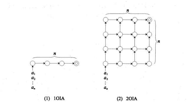
One of the simplest models of parallel computation is the one-way iterative array (OIA) [2, 3]. Figure 1 shows one-dimensional iterative array (IOIA) and two-dimensional iterative array
$(2\mathrm{O}\mathrm{I}\mathrm{A})$. These lower-dimensional arrays can be generalized to $k$ dimensions $(k\geq 1)$, i.e.,
to a $k$-dimensional one-way iterative array $(k\mathrm{O}\mathrm{I}\mathrm{A})$. Such an array has size $n\mathrm{x}\cdots\cross n(k$
times). The input cell is at position (1,$\ldots$, 1) and the accepting cell is at position $(n, \ldots , n)$
.
A $k\mathrm{O}\mathrm{I}\mathrm{A}$ operates in time $T(n)$ is denoted by
$k\mathrm{O}\mathrm{I}\mathrm{A}(T(n))$. Let $k\mathrm{O}\mathrm{I}\mathrm{A}(T(n))$ denote the class of
languages accepted by $k\mathrm{O}\mathrm{I}\mathrm{A}(T(n))\mathrm{S}$. Forspecialcomplexity$\mathrm{f}\mathrm{u}\mathrm{n}\mathrm{c}\mathrm{t}\mathrm{i}_{0}\mathrm{I}\mathrm{o}\mathrm{e}$, define opt $=(k+1)n-k$, $k \mathrm{O}\mathrm{I}\mathrm{A}(\mathrm{l}\mathrm{i}\mathrm{n}\mathrm{e}\mathrm{a}\mathrm{r})--\bigcup_{c>0^{k\mathrm{o}}}\mathrm{I}\mathrm{A}(\mathrm{o}\mathrm{P}^{\mathrm{t}}+cn)$, and $k\mathrm{O}\mathrm{I}\mathrm{A}(\mathrm{P}^{\mathrm{o}}1\mathrm{y}- l)=k\mathrm{O}\mathrm{I}\mathrm{A}(\mathrm{o}\mathrm{p}\mathrm{t}+n^{l})$. Note that time
complexity is at least $(k+1)n-k$ for any $k\geq 1[2,6]^{\uparrow}$. Meanwhile, multihead finite automata
has being studied especially from theoretical interest $[4, 11]$ as a simplest extension of finite
automaton. A $k$-head
finite
automaton is a finite-state automaton with $k$-heads on a singleread-only input tape. Let $1\mathrm{A}\mathrm{F}\mathrm{A}(k)(1\mathrm{N}\mathrm{F}\mathrm{A}(k))$ denote the class of languages accepted by
one-way $k$-head alternating (nondeterministic) finite automata. We denote the two-way version
of $1\mathrm{A}\mathrm{F}\mathrm{A}(k)$ by $2\mathrm{A}\mathrm{F}\mathrm{A}(k)$. As
a
relationship between multihead finite automata and one-wayiterative arrays, it is known [6] that $1\mathrm{N}\mathrm{F}\mathrm{A}(k+1)\subseteq k\mathrm{O}\mathrm{I}\mathrm{A}(\mathrm{o}\mathrm{p}\mathrm{t})$ for each $k\geq 1$. Section 3 cf
this paper generalizes it to the best result IAFA$(k+1)^{\mathrm{R}}=k\mathrm{O}\mathrm{I}\mathrm{A}(\mathrm{o}\mathrm{p}\mathrm{t})$, where $‘ \mathrm{R}$’ stands for
reversal operation.
Oneof the well-known$‘ 0$
pen problems
concerriing
to $\dot{\mathrm{O}}\mathrm{I}\dot{\mathrm{A}}$is whether IOIA$(\mathrm{o}\mathrm{p}\mathrm{t})\wedge\subset+\mathrm{l}\mathrm{O}$IA(linear).
Section4 of this paper connects this problem to AFA-side open problems whether IAFA(2)
$+\subset 2\mathrm{A}\mathrm{F}\mathrm{A}(2)$ andwhether IAFA(2) $+\subset$ IAFA(3), byshowing that$k\mathrm{O}\mathrm{I}\mathrm{A}(\mathrm{l}\mathrm{i}\mathrm{n}\mathrm{e}\mathrm{a}\mathrm{r})=1$-turn $2\mathrm{A}\mathrm{F}\mathrm{A}(k+$
$1)=$ finite-turn $2\mathrm{A}\mathrm{F}\mathrm{A}(k+1)\subseteq 1\mathrm{A}\mathrm{F}\mathrm{A}(k+2)$, where “1-turn” of $2\mathrm{A}\mathrm{F}\mathrm{A}(k)$ means that only
one
head among the $k$ headscan
turn at the right end of the input andmove
to the left, whileall the other heads must stop after arriving at the right end, starting at the left end. The term
“finite-turn”
means
that the number of full scans ofeach two-way head between both ends ofthe input (i.e., from the left end to the right end
or
vice versa) is restricted to be finite. This section also shows that $k\mathrm{O}\mathrm{I}\mathrm{A}(\mathrm{P}^{\mathrm{o}}1\mathrm{y}- l)\subseteq 2\mathrm{A}\mathrm{F}\mathrm{A}(k+l)$ ..
Section 6
summari.zes
the paper withconclu.d
$\mathrm{i}\mathrm{n}\mathrm{g}$remarks.$\underline{n}$
$n$
$-n$
(1) IOIA (2) $2\mathrm{O}\mathrm{I}\mathrm{A}$
Figure 1. One-dimensional and two-dimensional one-way iterative arrays.
2.
Definitions
“Unrolling” the computation of a $k\mathrm{O}\mathrm{I}\mathrm{A}$ in space and time $[1, 5]$,
we
obtainan
array ofcombi-national circuits: the $(k+1)$-dimensional trellis automaton.
Definition 2.1. A $(k+1)$-dimensional trellisautomaton$(k\mathrm{T}\mathrm{A})$ is
a
system$A=(\mathrm{E}, \Gamma, \Sigma, \Delta, f)$,where $\mathrm{E}$ is the
non-zero
quadrant$\{(i_{0}, i_{1}, \ldots, ik)\in \mathbb{Z}^{k+1}|i_{0}, i_{1}, \ldots, i_{k}\geq 0\}$ of $(k+1)-$
dimensional discrete space $\mathbb{Z}^{k+1}$. At each point $(i_{0}, i_{1}, \ldots , i_{k})$
of$\mathrm{E}$, an identicalelement, called
$(i_{0}, i_{1}, \ldots , i_{k})$-element, computes a partial function $f$ : $\Gamma^{k+1}arrow\Gamma$, where $\Gamma$ (which contains the
blanksymbol $\lambda$) is afinite operational alphabet. Output
$s$($i0,$il,$\ldots$,$i_{k}$) of$(i_{0}, i_{1}, \ldots , i_{k})$-element
is recursively defined: $s(i_{0}, i_{1}, \ldots, ik)=f(s0, S_{1}, \ldots, Sk)$, where $s_{0}--s(i_{0}-1, i_{1}, \ldots , i_{k}),$ $s_{1}$ –
$s(i_{0}, i_{1}-1, \ldots, i_{k}),$
$\ldots\}$and $s_{k}=s(i_{0}, i_{1}, \ldots, ik-1)$, with boundary condition$s(\mathrm{O}, i_{1}, i_{2}, \ldots, ik)=$
$s(i0,0, i_{2}, \ldots , i_{k})=\cdots=s(i_{0}, i1_{)}\cdots, ik-1,0)=\lambda$foreach$i_{0},$ $i_{1},$
$\ldots,$$i_{k}\geq 1$ exceptthat$s(i_{0},1,$$\ldots$ ,
1,$0$) $=a_{i_{0}},1\leq i_{0}\leq n$. We says that $A$ accepts input $a_{1}a_{2}\ldots a_{n}\in\Sigma^{*}$ in time $T(n)$ if
$s(T(n), n, \ldots , n)\in\Delta$, where $\Sigma,$$\Delta\subseteq\Gamma-\{\lambda\}$
are
the sets of input symbol8 and accepting$symb_{\mathit{0}}l\mathit{8}$, respectively.
Let $(k+1)\mathrm{T}\mathrm{A}(T(n))$ denote a $(k+1)\mathrm{T}\mathrm{A}$operates in time $T(n)$ and $(k+1)\mathrm{T}\mathrm{A}(T(n))$ denote
the class of languages accepted by $(k+1)\mathrm{T}\mathrm{A}(T(n))’ \mathrm{s}$. Figure 2 illustrates $2\mathrm{T}\mathrm{A}(T(n))$. It isclear
that $(k+1)\mathrm{T}\mathrm{A}(\tau(n))=kO\mathrm{I}\mathrm{A}(T(n))$ for any $k\geq 1$ and any $T(n)\geq(k+1)n-k$ .
Next, weintroduce
a
varietyof alternating multihead finite automaton, ranging from ordinaryone-way machine to two-way
one
[11]. Wefirst define the most general type of multihead finiteautomaton: the two-way alternating finite automaton.
Definition 2.2. An altemating
finite
automaton with $k$ head8 $(\mathrm{A}\mathrm{F}\mathrm{A}(k))$ is a structllre $M=$$(Q, \Sigma, \delta, q0, U, F)$, where (1) $Q$ is afinite, nonempty set of states; (2) $\Sigma$ is theinput alphabet $(\Sigma$
does not contain the symbols$\phi$ and
$);
(3) $\delta$isthe transition function, mapping$Q\cross(\Sigma\cup\{\psi, })^{k}$into the subsets of$Q\cross\{-1,0, +1\}^{k}$, withthe restriction that for any transition $(q, (d_{1}, \ldots, d_{k}))\in$
$\delta(p)(a_{1}, \ldots, a_{k})),$ $a_{j}=\phi$ implies $d_{j}\geq 0$ and $a_{j}=$ implies $d_{j}\leq 0$ for any $j(1\leq j\leq k);(4)$ $q_{0}\in Q$ is the initial state; (5) $U\subseteq Q$ is the set of universal states; and (6) $F\subseteq Q$ is the set of
$n$ $T(n)$
Figure 2. $2\mathrm{T}\mathrm{A}(T(n))$.
The language accepted by $M$ is $L(M)=$
{
$x\in\Sigma^{*}|M$ accepts $x$}.
The class of languagesaccepted by $\mathrm{A}\mathrm{F}\mathrm{A}(k)’ \mathrm{s}$ is denoted by $\mathrm{A}\mathrm{F}\mathrm{A}(k)$.
We next introduce special types of$\mathrm{A}\mathrm{F}\mathrm{A}(k)$ whose input heads are restricted in various ways.
A $\mathit{8}weeping$ head is a two-way head whose motions are restricted to be sweeping ones between
both ends of the input (i.e., from the left end to the right endor viceversa). A
finite-tum
head isa
sweeping head whose number of sweeps is restricted to be finite. A l-tum head $(l\geq 0)$ isa finite-turn head which
can reverse
its direction at most $l$ times. A $\mathit{0}$ne-way head is an aliasof$0$-turn head. An AFA$(k)$ with $k_{0}$ two-way heads, $k_{1}$ sweeping heads, $k_{2}$ finite-turn heads, $k_{3}$ $1$-turn heads, and $k_{4}$ one-way heads is denoted by $\mathrm{A}\mathrm{F}\mathrm{A}(k_{0}+\overline{k_{1}}+\overline{k_{2}}+\overline{k_{3}}+arrow k_{4})$.
Thesuperscript $‘ \mathrm{b}$’ of head notionimpliestheir blindne88, i.e., they cannot read inputsymbols
except the left and right boundary symbols $\phi$ and
$,
respectively $[4, 12]$.3.
Optimal-Time
$k\mathrm{O}\mathrm{I}\mathrm{A}$In this section,
we
shows the equivalence ofoptimal-timeOIA andone-wayAFA through reversal operationoflanguages. In order to clarifyourproofs, weintroduceaspecial typeofheadofAFA,a $reversal_{-}one$-way head which can move right-to-left, rather than left-to-right as an ordinary
one-way head. An$\mathrm{A}\mathrm{F}\mathrm{A}(k)$ with $k’$ $\mathrm{r}\mathrm{e}\mathrm{v}\mathrm{e}\mathrm{r}\mathrm{S}\mathrm{a}1_{-_{\mathrm{o}\mathrm{n}}}\mathrm{e}$-way heads is denoted by $\mathrm{A}\mathrm{F}\mathrm{A}(\cdots+k’arrow+\cdots)$. It
is clear that $\mathrm{A}\mathrm{F}\mathrm{A}(k)arrow=\mathrm{A}\mathrm{F}\mathrm{A}(k)^{\mathrm{R}}arrow$ and $\mathrm{A}\mathrm{F}\mathrm{A}(1arrow+\mathrm{b}^{arrow}k)=\mathrm{A}\mathrm{F}\mathrm{A}(1arrow+arrow k^{\mathrm{b}})^{\mathrm{R}}$.
Lemma 3.1. For each $k\geq 1,$ $k\mathrm{O}\mathrm{I}\mathrm{A}(\mathrm{o}\mathrm{p}\mathrm{t})\subseteq \mathrm{A}\mathrm{F}\mathrm{A}(1arrow+\mathrm{b}^{arrow}k)$
.
Proof. Let $A=(\mathrm{E}, \Gamma, \Sigma, \Delta, f)$ be a $(k+1)\mathrm{T}\mathrm{A}(\mathrm{o}\mathrm{p}\mathrm{t})$ equivalentto a$k\mathrm{O}\mathrm{I}\mathrm{A}(\mathrm{o}\mathrm{p}\mathrm{t})$ accepting
some
language $L$. It is easily
seen
that, givenan
i.n
put$a_{1}\ldots a_{n}.$’ each $(i, 1, \ldots, 1)$-element $(1 \underline{<}i\leq n)$
of $A$ can distribute its input symbol $a_{i}$ to all the elements having the same $i$-coordinates. We
$\mathrm{t}\mathrm{h}\mathrm{e}\mathrm{r}\mathrm{e}\dot{\mathrm{f}}\mathrm{o}\mathrm{r}\mathrm{e}$
assume that the initial condition of $A$ is the following: For each $1\leq i,$$i_{1},$
$\ldots,$$i_{k}\leq n$, $s(\mathrm{O}, i_{1}, i_{2}, \ldots , i_{k})=\lambda$, and $s(i, \mathrm{o}, i_{2}, \ldots , i_{k})=s$($i,$il,$0,$
$\ldots,$$ik$) $=\cdots=S$($i,$il,$\ldots$ ,$i_{k-1)}\mathrm{O}$) $=ai$.
Consider an $\mathrm{A}\mathrm{F}\mathrm{A}(1arrow+\mathrm{b}^{arrow}k)M=(Q, \Sigma, \delta, q_{0}, U, F)$ which executes the program shown in
Fig. 3
on a
tape$x$.
Wecan
imagine $M$to be anordinaryone-head finite $\mathrm{a}\mathrm{u}\mathrm{t}\mathrm{o}\mathrm{m}\mathrm{a}\mathrm{t}\mathrm{o}\mathrm{n}$ ’whose input tape $x$ is
a
$(k+1)$-dimensional ‘hyper-rectangle.’ Correctness of the algorithmcan
be proved byinduction as in the same way with that ofProposition 3.1 in [10]. We therefore conclude that
Main program
$\mathrm{b}\mathrm{e}\mathrm{g}\mathrm{i}\mathrm{n}//\mathrm{s}\mathrm{t}\mathrm{a}\mathrm{r}\mathrm{t}$from the right boundary sylnbol
$//
moves all headsonesquareleft (to the last symbol of$x$);
guess $s_{\mathrm{a}}\in\Delta$;
OUTPUT$(s_{\mathrm{a}})$
end
Procedure OUTPUT$(\dot{s})$
begin
ifsomehead reaches $\phi$ and reading head $h_{0}$ reads $\dot{s}$
thenacceptelsereject and halt
else
guess$s_{0},s_{1},$$s2,$$\ldots,sk\in\Gamma$ in such a way that $\dot{s}=f(s_{0},\dot{S}_{1}, s_{2}, \ldots , s_{k})$;
for each$j(0\leq j\leq k)$ dothefollowing in universal branching
begin
moves head $h_{j}$ one squareto the left;
OUTPUT$(_{S_{j}}.)$
end
end
Figure 3. Algorithm of reversal-one-way AFA simulating a OIA.
Lemma 3.2. For each $k\geq 2,$ $\mathrm{A}\mathrm{F}\mathrm{A}(k)arrow\subseteq(k-1)\mathrm{O}\mathrm{I}\mathrm{A}(0_{\mathrm{P}^{\mathrm{t})}}$
.
Proof. Ourtechnique is essentially thesame as that tlsed in the proofof Theorem 6.2 in [11], i.e., ‘reverse breadth-first search’ of the directed graph induced from all possible configuratiolls of an AFA.
Without loss of generality, we impose the following assumptions on any $\mathrm{A}\mathrm{F}\mathrm{A}(k)arrow M=$
$(Q, \Sigma, \delta, q0, U, F),$ $k\geq 2$.
(1) Initially, all heads of $M$ stay at the one left square to the right boundary symbol $, i.e.,
the initial configuration of$M$ on a tape $x$ is $(q_{0)}(n, n, \ldots, n))$, where $n=|x|$.
(2) At each step, any two heads of$M$doesnot moveleft simultaneously. From this, wemodify
the original transition function $\delta$ of$M$ to be
a
mapping $\delta’$ from$Q\cross(\Sigma\cup\{})^{k}$ into the
subsets of$Q\mathrm{x}\{0,1,2, \ldots , k\}$, where $(q, h)\in\delta’(p, a)$ implies atransition such that the $h\mathrm{t}\mathrm{h}$
head
moves
right and all other heads keep stationary (especially $h=0$ means all heads stationary).(3) If
some
head reaches$\phi$, allheads keep stationary afterward, i.e., $(q, h)\in\delta’(p,$$(a_{1},$
$\ldots,$$\phi,$ $\ldots$,
$a_{k}))$ implies $h=0$. This is possible because we can modify $M$ to the desired machine $M’$
as follows. Each time when
some
head $h$ of$M$ is going tomove
left, $M’$ guesses whetherthe symbol of the square that $h$ will enter is $\phi$ or not and universally branches into two
machines, one of which really
moves
$h$ to the left and checks the correctness of the guess(and halts), other of which continues the simulation of$M$, assuming$\phi$ onthe left neighbor
square (and keeping $h$ stationary).
Let $M’=(\{q_{0}, q_{1}, \ldots, qS\}, \Sigma, \delta/,Uq_{0},, F)$be an $\mathrm{A}\mathrm{F}\mathrm{A}(k)arrow$
which satisfies the above-mentioned
conditions. Prior to the simulation of $M’$, we prepare a look-up table $g$ : $(\{0,1\}S+1)^{k}\cross$
$(\Sigma\cup\{})^{k}arrow\{0,1\}^{S}+1$, which is constructed by the algorithm shown in Fig. 4.
. Note that the algorithm only
uses
the information of $M’$, not of individual input string andthat the resultant table $g$ is offinite memory size.
Consider
a $k\mathrm{T}\mathrm{A}A=(\mathrm{E}, \Gamma, \Sigma, \Delta, f)$ ona
tape $x=a_{1}a_{2}\ldots a_{n}$. By using a standard ‘folding’Procedure$g(u^{(1)}, u(2),$$\ldots u^{(k}\rangle,$$a)$ begin
for each$r(0\leq r\leq \mathit{8})$ initialize $u_{r}^{(0)}:=\{$ 1, if
$q_{r}\in F$,
$0$, otherwise.
repeat $s$ times do begin
for each$r’ \mathrm{s}(0\leq r\leq s)$ such that $u_{r}^{(0)}=0$do
begin
if$q_{r}\in U$ then
if
for
allpair $(l, h)(0\leq l\leq s, 0\leq h\leq k)$ such that $(q_{l}, h)\in\delta’(q_{r}, a)$, it holds that $u_{l}^{(h)}=1$ then$u_{r}^{(0)}:=1$$\mathrm{e}\mathrm{l}\mathrm{s}\mathrm{e}//q_{r}\in Q-U//$
if at least one pair $(l, h)(0\leq l\leq \mathit{8},0\leq h\leq k)$ such that $(q_{l}, h)\in\delta’(q_{r}, a)$, it holds that $u_{l}^{(h)}=1$ then$u_{r}^{(0)}:=1$
end end
return$u^{(0)}=(u_{0}^{(0)}, u^{(0},., u_{s})1)..(0)$
end
Figure 4. Construction algorithm oflook-up table $g$ of
$\mathrm{A}\mathrm{F}\mathrm{A}(k)arrow$
.
$(a_{i_{1}}, a_{i}2)\ldots$,$a_{i_{k}}$) of input $x$ is available for each $(i_{1}, i_{2}, \ldots, i_{k})$-element of $A(1\leq i_{1},$
$i_{2},$
$\ldots,$$i_{k}\leq$
$n)$. The operational function $f$ of$A$ with such a distributed input is thus defined
as
follows.For each$1\leq i_{1},$$i_{2},$
$\ldots$,$i_{k}\leq n,$
$(i_{1}, i_{2}, \ldots, i_{k})$-element outputs the vector$v^{(0)}=g(v(1), v(2)$,
. . .,$v^{(k)},$ $(a_{i_{1}}, a_{i_{2}}, \ldots, a_{i})k)$, where $v^{(1)}$ is the input vector from $(i_{1}-1, i_{2}, \ldots , i_{k})$-element,
$v^{(2)}$ is the input vector from $(i_{1}, i_{2}-1, i_{3,\ldots,k}i)$-element, .. . , and $v^{(k)}$ is the input vector
from $(i_{1}, i_{2}, \ldots, i_{k-}1, ik-1)$-element except that when$i_{j}=1,$ $v^{(}j$) $=g(v^{*}\ldots,$$v^{*})’(a_{1},$ $\ldots$,
$j\emptyset^{\downarrow},$
. . .,$a_{k}$)), where $‘ v^{*}’$ stands for an arbitrary (don’t-care) vector.
Recall from the assumption (3) that all heads stop their motions after some head reaches $\phi$, so the actual values of parameters $u’ \mathrm{s}$ have no relevance to the reference of $g$ when another
parameter $a$ contains symbol $\phi$.
Correctness of the whole algorithm
can
be proved by induction as in thesame
way with that ofProposition 3.2 in [10]. Therefore, we canconclude that $A$ accepts the same language as $M’$.It followsthat a $(k-1)\mathrm{o}\mathrm{I}\mathrm{A}(\mathrm{o}\mathrm{P}^{\mathrm{t})}$ equivalent to $A$ accepts $L(M’)$.
$\square$
FromLemma 3.1 and 3.2, we get the main theorem of this section.
Theorem 3.1. For each $k\geq 1,$ $k\mathrm{O}\mathrm{I}\mathrm{A}(\mathrm{o}\mathrm{p}\mathrm{t})\mathrm{R}\mathrm{A}\mathrm{F}\mathrm{A}=(1arrow+\vec{k}^{\mathrm{b}})=\mathrm{A}\mathrm{F}\mathrm{A}(k+arrow 1)$ . $\square$
4.
Linear-Time
and Polynomial-Time
$k\mathrm{O}\mathrm{I}\mathrm{A}’ \mathrm{s}$In this section, we investigate the relationships between $\mathrm{n}\mathrm{o}\mathrm{n}- \mathrm{O}\mathrm{P}^{\mathrm{t}\mathrm{i}1_{-}\mathrm{t}\mathrm{i}}\mathrm{m}\mathrm{a}\mathrm{m}\mathrm{e}$ OIA’s and AFA’s.
Notably, we show that linear-time OIA’s are completely characterized with finite-turn AFA’s. Almost proofs
are
based on the characterizationoftime-bounded OIA interms ofaspecial typeof
one-way.
AFA.Definition 4.1. For any language $L$ and any non-negative function $T(n)$, define $L\#^{\tau(n)}=$
$\{x\#^{T(n})|x\in L\}$ and $\#^{T(n)}L=\{\#^{\tau(}n)_{X}|x\in L\}$, where $\#$ is not in the alphabet of$L$.
In the below, superscript “
$\#$” on
$\vec{k}$
means that the corresponding $\vec{k}$
heads imitially stay at the rightnlost symbol ofpadding substring $\#^{7}\mathrm{s}$, i.e.,
one
square left to substring $x$.As aneasygeneralizationof Theorem 3.1, wehave the following characterization of arbitrary-time bounded OIA (recall that $L\#^{0}=L$).
Theorem 4.1. Let$L$ be any language and$T(n)$ be any non-negative
function.
Then,for
each$k\geq 1,$ $L\in k\mathrm{O}\mathrm{I}\mathrm{A}(\mathrm{o}\mathrm{p}\mathrm{t}+T(n))\Leftrightarrow\#^{T(n})L^{\mathrm{R}}\in \mathrm{A}\mathrm{F}\mathrm{A}(1+arrow\#_{\vec{k}^{\mathrm{b}})}$. $\square$
By using the above characterization,weget thefollowing speed-up theorem formulti-dimensional
OIA, which includes one- and two-dimensional versions $[7, 8]$ as special cases. Theorem 4.2 ($\mathrm{m}\mathrm{u}\mathrm{l}\mathrm{t}\mathrm{i}-\mathrm{d}\mathrm{i}\mathrm{m}\mathrm{e}\mathrm{n}\mathrm{S}\mathrm{i}\mathrm{o}\mathrm{n}\tilde{\mathrm{a}}1$
speed-up). Let $T(n)$ be any non-negative
function
and$d>0$ be any constant. Then, $k\mathrm{O}\mathrm{I}\mathrm{A}(\mathrm{o}\mathrm{p}\mathrm{t}+T(n))=k\mathrm{O}\mathrm{I}\mathrm{A}(\mathrm{o}\mathrm{p}\mathrm{t}+T(n)/d)$
for
each $k\geq 1$.Proof. From Theorem4.1, it is sufficient to show that $\#^{T(n)}L\in \mathrm{A}\mathrm{F}\mathrm{A}(1+arrow\#_{\vec{k}^{\mathrm{b}}})\Rightarrow\neq^{T(n)}/dL\in$
$\mathrm{A}\mathrm{F}\mathrm{A}(1arrow+\#_{\vec{k}^{\mathrm{b}})}$. Let $M$
be
an
$\mathrm{A}\mathrm{F}\mathrm{A}(1arrow+\#_{\vec{k}^{\mathrm{b}})}$ accepting $\#^{T(n)}L$. An $\mathrm{A}\mathrm{F}\mathrm{A}(1arrow+\#_{\vec{k}^{\mathrm{b}})}M’$ that
simulates $M$ behaves in the
same
way as $M$, except when the reading head $h$ of $M$ is onpaddingsymbols $\#’ \mathrm{s}$of the given tape: Each time $h$
moves
$d$squares to the right, $M’$moves
itsreading head $h’$ one square to the right. It is clear that $M’$ accepts $\#^{\tau(n)/}dL$.
$\square$
Substituting$T(n)=dn$,
we
have the speed-up theorem in linear-time range.Corollary 4.1. For each $k\geq 1,$ $k\mathrm{O}\mathrm{I}\mathrm{A}(\mathrm{l}\mathrm{i}\mathrm{n}\mathrm{e}\mathrm{a}\mathrm{r})=k\mathrm{O}\mathrm{I}\mathrm{A}(\mathrm{o}\mathrm{p}\mathrm{t}+n)$ . $\square$
This fact will be used in the following discussions. In the case of linear-time OIA, we can
relax the
restriction..
ofinitial head positions on the equivalent one-way AFA:Proposition 4.1. Let $L$ be any language. Then,
for
each $k\geq 1,$ $\neq^{n}L\in \mathrm{A}\mathrm{F}\mathrm{A}(1arrow+\#_{\vec{k}^{\mathrm{b}})}\Leftarrow\Rightarrow$ $\#^{n_{L\in \mathrm{A}\mathrm{F}\mathrm{A}}}(1+\vec{k}\mathrm{b})arrow$.$\square$
Thefollowing pairof lemmas leads to the theorem which asserts theequivalenceof linear-time
OIA and finite-turn AFA.
Lemma 4.1. For each $k\geq 1,$ $k\mathrm{O}\mathrm{I}\mathrm{A}(\mathrm{o}_{\mathrm{P}}\mathrm{t}+n)^{\mathrm{R}}\underline{\subseteq}\mathrm{A}\mathrm{F}\mathrm{A}(\hat{1}+\vec{k}^{\mathrm{b}})$
.
Proof. From Theorem 4.1 and Proposition 4.1, it is sufficient to show that $\#^{n}L\in \mathrm{A}\mathrm{F}\mathrm{A}(1arrow+$
$\vec{k}^{\mathrm{b}})\Rightarrow L\in \mathrm{A}\mathrm{F}\mathrm{A}(\hat{1}+\vec{k}^{\mathrm{b}})$
. Let $M$be an$\mathrm{A}\mathrm{F}\mathrm{A}(1+\vec{k}\mathrm{b})arrow$accepting
$\neq^{n}L$. We constructan$\mathrm{A}\mathrm{F}\mathrm{A}(\hat{1}+\vec{k}^{\mathrm{b}})$
$M’$ which acts
as
follows. $M’$ behaves in thesame
way as $M$, except thatsome
blind head $b’$ isused for the reading head $r$ of $M$ (and its reading head $r’$ is used for the corresponding blind
head $b$ of $M$). When $b’$ wants to read input symbol, $M’$ performs a
$\mathrm{g}\mathrm{u}\mathrm{e}\mathrm{S}\mathrm{S}^{- \mathrm{a}\mathrm{n}}\mathrm{d}$-check procedure $\mathrm{s}\mathrm{i}\mathrm{m}L$
.
ilarto that used in the assumption (3) of the proof ofLemma 3.2. It is clear that $M’\mathrm{a}\mathrm{C}\mathrm{C}\mathrm{e}\mathrm{p}\mathrm{t}\mathrm{S}\square$
Lemma 4.2. For each $k\geq 1,$ $\mathrm{A}\mathrm{F}\mathrm{A}(k\overline{+}1)\subseteq k\mathrm{O}\mathrm{I}\mathrm{A}(\mathrm{o}_{\mathrm{P}}\mathrm{t}+n)$
.
Proof. Indirect simulation using one-way AFA $(\mathrm{T}\underline{\mathrm{h}\mathrm{e}}\mathrm{o}\mathrm{r}\mathrm{e}\mathrm{m}4.1)$ arerathercomplicated. Instead, we briefly describe the direct sinlulation of $\mathrm{A}\mathrm{F}\mathrm{A}(k+1)$ by $k\mathrm{O}\mathrm{I}\mathrm{A}(\mathrm{o}\mathrm{p}\mathrm{t}+n)$. Figure 5 illustrates
a
trellis automaton equivalent to a $1\mathrm{O}\mathrm{I}\mathrm{A}(\mathrm{o}\mathrm{p}\mathrm{t}+n)$ that simulates an $\mathrm{A}\mathrm{F}\mathrm{A}(\tilde{2})$ whose first headis 1-tum and second is 2-turn. The shaded
area
in the figure is used for actual simulation.The remaining part is used only for sending the input information to the simulation
area.
Thedetailed construction is omitted. $\square$
From Lemma 4.1 and Lemma 4.2, we have the followingequivalence.
Theorem 4.3. For each $k\geq 1,$ $k\mathrm{O}\mathrm{I}\mathrm{A}(1\mathrm{i}\mathrm{n}\mathrm{e}\mathrm{a}\mathrm{r})=\mathrm{A}\mathrm{F}\mathrm{A}(k\overline{+}1)=\mathrm{A}\mathrm{F}\mathrm{A}(\hat{1}+\vec{k}^{\mathrm{b}})$.
$a_{1}$ $a_{2}$
’... $a_{n}.$
.
$n$
Figure 5. Simulation of$\mathrm{A}\mathrm{F}\mathrm{A}(\tilde{2})$ by $1\mathrm{O}\mathrm{I}\mathrm{A}(\mathrm{o}\mathrm{P}^{\mathrm{t}}+n)$.
Exchanging the blindness of zero-turn head and non-zero-turn heads of $\mathrm{A}\mathrm{F}\mathrm{A}(\hat{1}+\vec{k}^{\mathrm{b}})$ (or
strengthening the one-way blind heads of $\mathrm{A}\mathrm{F}\mathrm{A}(1arrow+\vec{k}^{\mathrm{b}})$ to finite-turn ones),
we.get
a refined hierarchy between $k\mathrm{O}\mathrm{I}\mathrm{A}(\mathrm{o}\mathrm{p}\mathrm{t})$ and $k\mathrm{O}\mathrm{I}\mathrm{A}(\mathrm{l}\mathrm{i}\mathrm{n}\mathrm{e}\mathrm{a}\mathrm{r})$:Theorem 4.4. $\mathrm{A}\mathrm{F}\mathrm{A}(1arrow+k-1^{\mathrm{b}}arrow+\wedge 1^{\mathrm{b}})=\mathrm{A}\mathrm{F}\mathrm{A}(\hat{1}^{\mathrm{b}}+\vec{k})=\mathrm{A}\mathrm{F}\mathrm{A}(1arrow+\tilde{k}^{\mathrm{b}})$ . $\square$
Next, we show that finite-turning ability of input heads can be discarded at the cost ofone
additional head.
Theorem 4.5. For each $k\geq 2,$ $\mathrm{A}\mathrm{F}\mathrm{A}(\tilde{k})\subseteq \mathrm{A}\mathrm{F}\mathrm{A}(k+1)arrow$.
Proof. From Theorem 3.1 and Theorem 4.3, it is sufficient to show that $\mathrm{A}\mathrm{F}\mathrm{A}(\vec{k}^{\mathrm{b}}+\hat{1})^{\mathrm{R}}\subseteq$ $\mathrm{A}\mathrm{F}\mathrm{A}(k^{\mathrm{b}}+\wedgearrow 2)$. Let $M$bean$\mathrm{A}\mathrm{F}\mathrm{A}(\vec{k}^{\mathrm{b}}+\hat{1})$ acceptingsomelanguage$L$. Weconstructan$\mathrm{A}\mathrm{F}\mathrm{A}(\vec{k}^{\mathrm{b}}+2)arrow$
$M’$which accepts $L^{\mathrm{R}}$
as
follows. The $\vec{k}^{\mathrm{b}}$heads of$M’$ behave in the
same
way as the$\vec{k}^{\mathrm{b}}$heads cf
$M$, except that they move in the reversal direction of that of$M$. The simulation of the $\hat{1}$
-type head $h$ of $M$ consists of two stages. Stage 1: Before $h$ turns at the left end of the input, $M’$
moves one of its 2 heads, say $h’$, in the same way as $h$ except that it moves in the reversal
direction, the remaining head $h^{\prime/}$ being kept stationary at the left end. When $b’$ wants to read
input symbol, $M’$ performs aguess-and-check procedure similar to that used in the assumption
(3) of the proof of Lemma 3.2. Stage 2: After $h$ turns at the left end ($h’$
:
arrives at the $\mathrm{r}\mathrm{i}\mathrm{g}\mathrm{h}\mathrm{t}\square$
end), $M’$ begins to move $h^{\prime/}$ to the right as $h$
moves
right.As
a
final result,we
show thata
polynomial-time $k\mathrm{O}\mathrm{I}\mathrm{A}$can
be simulated bya
two-way$(l+k)$-head AFA, where $l$ is the degree of the polynomial.
Theorem 4.6. For each $k,$$l\geq 1,$ $k\mathrm{O}\mathrm{I}\mathrm{A}(\mathrm{P}^{\mathrm{o}}1\mathrm{y}- l)\subseteq \mathrm{A}\mathrm{F}\mathrm{A}(\overline{l-1}+k+1^{\mathrm{b}})arrow$. $\square$
5.
Conclusion
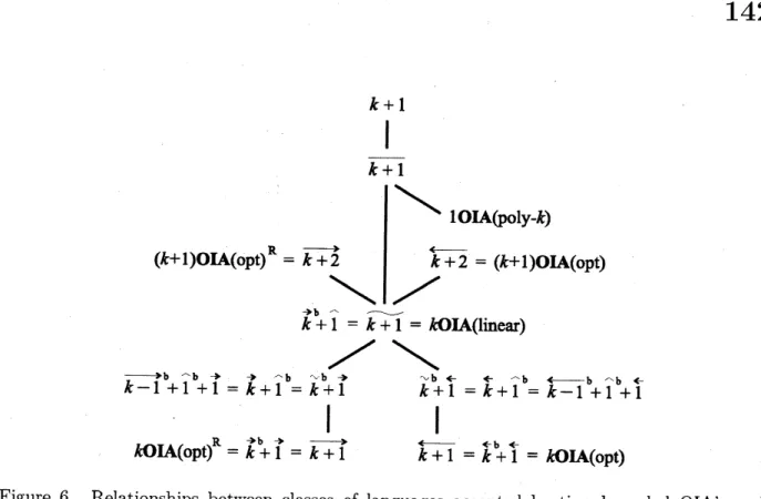
Figure 6summarizes the main results obtained in thispaper. In the figure,
we
are
omitting prefix “AFA” fromlanguageclassnotation ofAFA’s, e.g., “$k+1$” isthe abbreviationof “$\mathrm{A}\mathrm{F}\mathrm{A}(k+1).$”
It is unknown whether any one of the inclusions is proper or not.
References
[1] C. Choffrut andK.CulikII, “Onreal time cellularautomataandtrellisautomata,” Acta
Infonnatica
21, pp.393-407 (1984).$k+1$
$\frac{1}{k+1}$
$(k+1)\mathrm{o}\mathrm{I}\mathrm{A}(\mathrm{o}\mathrm{p}\mathrm{t})=\mathrm{n}k+2arrow$
$\wedge\backslash |_{/^{k+2}}^{\backslash _{1\mathrm{o}\mathrm{I}}}arrow=\mathrm{A}(\mathrm{p}\mathrm{o}(k+1\mathrm{y}1-)\mathrm{o}\mathrm{I}\mathrm{A}(\mathrm{o}k)\mathrm{p}\mathrm{t})$
$\overline{k}^{>\mathrm{b}}+1=\overline{k+}\overline{1}=k\mathrm{O}\mathrm{I}\mathrm{A}(\mathrm{l}\mathrm{i}\mathrm{n}\mathrm{e}\mathrm{a}\mathrm{r})$
$/$
$\backslash$$k-1^{\mathrm{b}}+1^{\mathrm{b}}arrow\wedge+1’=-k’+1^{\mathrm{b}}=\wedge k+1\sim \mathrm{b}arrow$ $\tilde{k}^{\mathrm{b}}+1arrow=k+1^{\mathrm{b}}=arrow\wedge k-1+arrow \mathrm{b}\wedge\iota\epsilon\iota+1$
$|$ $|$
$k\mathrm{O}\mathrm{I}\mathrm{A}(\mathrm{o}\mathrm{p}\mathrm{t})=k^{\mathrm{b}}+1\mathrm{R}arrowarrow=\overline{k+1}$
$\overline{k+1}=k^{\mathrm{b}}+1\epsilon\epsilon=k\mathrm{O}\mathrm{I}\mathrm{A}(\mathrm{o}\mathrm{p}\mathrm{t})$
Figure 6. Relationships between classes of languages accepted by time-bounded OIA’s and
multihead AFA’s $(k\geq 1)$.
[2] J. H. Chang, O. H. Ibarra, and A. Vergis, “On the power ofone-waycommunication,” JACM35,
No.3, pp.697-726 (1988).
[3] J. Gruska, “Synthesis, structure and power of systolic computations,” Theoret. Comput. Sci. 71, pp.47-77 (1990).
[4] J. Hromkovic, “On the power ofalternation in automata theory,” JCSS31, pp.28-39 (1985).
[5] O. H. Ibarra, S. M. Kim, and S. Moran, “Sequentia} lnachinecharacterization oftrellis and cellular automataand applications,” SIAMJ. Comput. 14, No.2, pp.426-447 (1985).
[6] O. H. Ibarra, “Systolic arrays: characterizations alld $\mathrm{c}\mathrm{o}\mathrm{m}\mathrm{p}\mathrm{l}\mathrm{e}\mathrm{x}\mathrm{i}\mathrm{t}\mathrm{y}_{)}’$
)
Proc. $MFCS’ s\mathit{6}$, LNCS 233,
pp.140-153 (1986).
[7] O. H. Ibarra, and T. Jiang, “On one-waycellulararrays,” SIAMJ. Comput. 16, No.6, pp.1135-1154
(1987).
[8] O. H. Ibarra and M. A. Palis, “
$\mathrm{T}_{\mathrm{W}\triangleright}\mathrm{d}\mathrm{i}\mathrm{m}\mathrm{e}\mathrm{n}\mathrm{S}\mathrm{i}\mathrm{o}\mathrm{n}\mathrm{a}1$ iterative arrays: characterizations
and
applica-tions,” Theoret. Comput. Sci. 57, pp.47-86 (1988).
[9] O.H.Ibarraand T.Jiang, $‘ \mathrm{t}\mathrm{R}\mathrm{e}\mathrm{l}\mathrm{a}\mathrm{t}\mathrm{i}\mathrm{n}\mathrm{g}$ thepowerof cellular arraystotheir cloeure
Properties,” Theoret.
Comput. Sci. 57, pp.225-238 (1988).
[10] A. Ito, K. Inoue, and I. Takanami, “Determinisitic two-dimensionalon-line tessellationacceptors are
equivalentto two-way two-dimensional alternating finite automata through 180-rotation,” Theoret.
Comput. Sci. 66, pp.273-287 (1989).
[11] K. N.King, “Alternatingmultihead finiteautomata,” Theoret. Comput. Sci. 61, pp.149-174 (1988).
[12] H. Matsuno, K. Inoue, H. Taniguchi, and I. Takanami, “Alternating simple multihead finite