Numerical methods for radiation and resonance problems (Numerical Solution of Partial Differential Equations and Related Topics)

Numerical methods for

radiation

and

resonance

problems

KAKO, Takashi (加古 孝) $*$

KANO, Tomotoshi (加納悶悶)

Department ofComputer Science

The University ofElectro-Communications

Chofu, Tokyo 182-8585, JAPAN

1

Introduction

The main purpose of this paper is to investigate some typical problems ofwave motion in

unbounded region which are related to radiation or scattering phenomena. The Helmholtz

equation is one of the most important mathematical models which is used to describe the

time harmonic behavior of various vibration and wave propagation phenomena.

The motivation of research is to understand main characteristics of wave propagation

phenomena in obstacle scattering $\mathrm{a}\mathrm{n}\mathrm{d}/\mathrm{o}\mathrm{r}$ wave radiation process through its numerical

computation based on its mathematical analysis.

The importance of the wavepropagation resides in the fact that it transmits information

and transports energy. Some examples of research fields related to the wave

propaga-tion include acoustics, elasticity, electromagnetism withvarious applications such as sound

emission from a speaker, human speech production, sound production of musical

instru-ments, noise reduction, diagnostics or detection by ultrasonic wave, propagation ofwaves

in optical fiber of fiber scope, heating by wave for various kinds of materials and others.

Some of the characteristic quantities to be calculated in these problems include scattering

amplitudes, transmission and reflection coefficients,

resonance

frequencies.

To investigate numerically the wave propagation phenomena in unbounded region using

computers, we have to approximate the original problem which is formulated in some

infinite dimensional function space by the one in an appropriate finite dimensional linear

space. For this purpose, we first use the knowledge of the analytical properties of the

solution to the original problem such as the radiation condition at infinity $\mathrm{a}\mathrm{n}\mathrm{d}/\mathrm{o}\mathrm{r}$ the

expression of the solution byaseries of specialfunctions or byan integral involving Green’s

function. Wethen reduce the problem intotheboundaryvalue problemin abounded region

with some truncation errorforitssolution and applya finite element discretization method to get the $\underline{1\mathrm{i}_{11}}\epsilon \mathrm{a}\mathrm{r}$ equation in a finite

dimensional

approximation space.

Especially, we will show the effectiveness of the radiation condition at infinity which

describes the asymptotic behavior of the solution and singles out the physical solution.

We then use the domain decomposition method which divides the original problem in an

unbounded region into the problem in a bounded region and the one in an outer region

with simple shape.

More specifically, we treat a two-dimensional wave-guide problem where we use the

exact boundary condition given by the Diriclet to Neumann map on the boundary between

a bounded region and

an

outer unbounded region which is cylindrical with a bounded

cross section. We also consider a one-dimensional problem related to this original

two-dimensional problem.

We

will show some numerical examples, and discuss the relationship between $2\mathrm{D}$ and

1D cases and show

some

numerical examples which indicate the efficiency of the 1D model

as the good approximation of the $2\mathrm{D}$ problem in the sense that it gives similar frequency

response

curves.

2

Mathematical

Formulation

The main mathematical framework of the study consists of the scattering theory based

on

the perturbation theory for linear operators and the finite element method for partial

differential. equations.

The first difficulty in

studyi.ng

the $\mathrm{r}\mathrm{a}.\mathrm{d}\mathrm{i}\mathrm{a}\mathrm{t}\mathrm{i}_{0}\mathrm{n}$ or scattering problem comes from the

un-boundedness of the region where we consider the partial differential $\mathrm{e}\mathrm{q}\mathrm{u}\mathrm{a}\mathrm{t}\grave{\mathrm{i}}_{\mathrm{o}\mathrm{n}}$and

we

have

to choose an appropriate function space. The second problem we have to $\dot{\mathrm{t}}\mathrm{r}\mathrm{e}\mathrm{a}\mathrm{t}$

appropri-ately is the indefiniteness of$\mathrm{t}\mathrm{h}\dot{\mathrm{e}}$

bilinear form which appears in the weak formulation used

for the finite element method in the artificial bounded region and we

_hav.e

to consider the

problem with non-real variables as well.

In this paper, werestrict ourstudytothe two-dimensional casealthoughthereal physical

phenomena occur in three-dimensional space. However, at least the theoretical part ofour

study can be extended to the three-dimensional case without any essential difficulty.

The

main problem we may have to solve is the practical computational complexity due to the

large number of unknowns in $3\mathrm{D}$ caseand the shortage ofmemoryand speed of the present

computers together with the human resources in programming.

2.1

Two-dimensional

Wave

Propagation

Problem

The wave propagation phenomena in two-dimensional space $R^{2}$ can be described by the

following mathematical model ofthe wave equation in $\Omega\subset R^{2}$:

$( \alpha\frac{\partial}{\partial n}+\beta)u(t,x, y)$ $=g(t,x,y)$

on

_{$(-\infty, \infty)\mathrm{x}\partial\Omega$},

(2)

where

$\frac{\partial}{\partial n}$ denotes

the

outward normal derivative

on

the boundary $\partial\Omega$ of $\Omega$

.

In the following,

we consider

a stationary

time

harmonic solution of theproblem: ,_$u(t,x,y)=$

$e^{i\omega t}u(x, y)$ for

inhomogeneous

data: _{$f(t,x,y)=e^{i\omega l}f(x,y)$} and _{$g(t, x,y)=e^{i\omega t}g(x, y)$} from

which

we

can

calculate almost

every

important quantity.

Then

$u$ satisfies the

Helmholtz

equation:

$(-\Delta-\omega^{2})u(X,y)$ $=f(x,y)$ in $\Omega$

,

(3)

$( \alpha\frac{\partial}{\partial n}+\beta)u(x,y)$ $=g(x,y)$

on

$\partial\Omega$ (4)

with

some radiation

condition at infinity $(r=(x^{2}+y^{2})^{1/2}arrow+\infty)$

.

We

assume

that the boundary $\partial\Omega$consists oftwo mutuallydistinct parts:

$\partial\Omega=\Gamma_{H}\cup\Gamma s$

where $g=g_{S}$

on

the

source

boundary $\Gamma_{S}$ and $g=0$

on

the

homogeneous boundary

$\Gamma_{H}$.

The existence and uniqueness of the

solution

to this

radiation

or

scattering problemcan be

proved by the limiting absorption principle

which

claims that the physical solution is the

limit

of the solution for the problem with positive absorption

when

the absorption tends

to

zero.

In case that

we

know

Green’s function of

the corresponding free space problem

which satisfies the radiation condition at infinity,

we

can construct the solution solvingthe

integral equation

on

the boundary.

2.2

Reduction

to

a

Problem

in a

Bounded Region

We introduce

an artificial

boundary in $\Omega$ which includes the

source

boundary

$\Gamma_{S}$ and we

assume

that the shape of the outside the boundary issimple. Forexample, it is the outside

of a disk or a cylindrical region. The, using the knowledge of the solution outside the

boundary we impose the boundary condition

on

the

artificial

boundary which may the

Diriclet to

Neumann

($\mathrm{D}\mathrm{t}\mathrm{N}$ in short) map

or

its approximation. We sometimes call

it a

radiation boundary

condition

(or artificial boundary condition).

In the $2\mathrm{D}$ wave-guide problem with a cylindrical unbounded

semi-infinite

channel, the

radiation condition in the cylindrical is

written as:

$\frac{\partial p}{\partial n}(=\frac{\partial p}{\partial x})=\Lambda p$ on

$\Gamma_{R}$

,

(5)

where

$\Gamma_{R}$ is

an

artificial boundary which is a

cross

section of the cylindrical region

and A

is the Dirichlet to

Neumann

nap in the outer cylindrical

region

given as

$\Lambda p=\sum_{\overline{\sim}^{0}}^{\infty}\gamma nCn(p)\mathrm{c}n\mathrm{o}\mathrm{s}(\frac{n\pi}{L}y)$ (6)

with

$C_{n}(p\rangle=\{$

$\frac{1}{L}\int_{0}^{L}p(x,y)dy$ $(n=0)$

$\frac{2}{L}\int_{0}^{L}p(x_{7}y)\cos(\frac{n\pi}{L}y)dy$ _{$(n\geq 1)$},

$\gamma_{n}=\{$ $i\zeta_{n}$, $-\eta_{n}$, $\zeta_{n}=\{\omega^{2}-(\frac{n\pi}{L})2\}^{1/}2$, $0< \frac{n\pi}{L}<\omega$ $\eta_{n}=\{(\frac{n\pi}{L})2-\omega 2\}^{1}/2$, $\omega\leq\frac{n\pi}{L}$. (8)

Then the Helmholtz equation in the inner domain $\Omega_{i}$ is given as:

$(-\omega^{2}-\Delta)p=0$ in $\Omega_{i}$ (9)

$\frac{\partial p}{\partial n}=0$ on

$\Gamma_{H}$, $\frac{\partial p}{\partial n}$

$=g_{S}$ on $\Gamma_{S}$

,

$\frac{\partial p}{\partial n}=\Lambda p$ on $\Gamma_{R}$

Related to

this

$2\mathrm{D}$ wave-guide problem, we can consider the corresponding

1D

Webster’s

horn equation given as:

$- \frac{\partial v}{\partial t}=\frac{A(x)}{\rho}\frac{\partial p}{\partial x’}$ $- \frac{\partial p}{\partial t}=\frac{\rho c^{2}}{A(x)}\frac{\partial v}{\partial x’}$ (10)

where$p$ is the pressureand $v$is the velocity, and$A(x)$ denotes the areaof the cross section.

Eliminating $v$, we have the 1D approximation model called Webster’s horn equation:

$\frac{\partial^{2}p}{\partial t^{2}}-\frac{1}{A(x)}c^{2_{\frac{\partial}{\partial x}(()\frac{\partial p}{\partial x})0}}AX=$, (11)

3

Week Formulation and

Discretization

In this paper, we use the finite element method to dicretize the problem in the artificially

truncated region with an artificial boundary condition. We start with a weak formulation

of the problem in an appropriate closed subspace $\mathcal{V}$ of the Sobolev space $H^{1}(\Omega_{i})$ defined

through the boundary condition and then restrict the problem into a finite dimensional

subspace of $\mathcal{V}$ which is a set of all piece-wise linear continuous functions in $\mathcal{V}$ with respect

to a regulartriangulation of$\Omega_{i}$

.

We note that we haveto introduce an appropriate

approx-imation of the boundary integral which corresponds to the non-local boundary condition

such as the higher order radiation boundary condition or the Dirichlet to Neumann map.

In the following, we show the case of the $2\mathrm{D}$ wave-guide problem in some detail.

The weak formulation for theHelmholtz problem (3) and (4) with the artificial boundary

condition is given as:

Find $p\in \mathcal{V}\subset H^{1}(\Omega)$ :

$a(p, q)=(f, q)(=a0(g, q))$ $\forall q\in \mathcal{V}$

where, together with its approximation $a_{N}(\cdot, \cdot)$,

$a(p, q)$ $=$ $a_{0}(p, q)+b_{1}(p, q)+b_{2}(p, q)$,

with

$a_{0\backslash }p,$$q’\backslash )$ $=$ $J_{\Omega}^{[_{\nabla_{\mathrm{v}}}}p\cdot\overline{\nabla q}|\perp p\overline{q}.d\tau_{U\prime}"\prime \mathrm{J}y$

$o(\iota_{1}p, q)$ $=$ $-/( \infty’+^{1}\perp)2\int_{\Omega}p\overline{q}dxdy$

$b_{2}(_{\sim^{\wedge}}p, q)$ $=$ $-(\Lambda p(_{X_{B}},$$\cdot \mathrm{I},$_{$q(xR, \cdot \mathrm{I})=b_{2}.;(p,$}

$q\mathrm{I}+b_{\underline{?},r}\infty(p,$ $q\mathrm{I}$

$U_{2,i(P,q}l/\backslash J$ $=$ _{$-i \omega LC_{0}(p)C_{0}(q)-\prime i0<\frac{\sum_{n\pi}}{L}<\omega\zeta_{n}(\frac{L}{2}JCn(p\backslash /)c_{n}(q)$}

$b_{2,r}^{\infty}(p, q)$ $= \sum_{\omega\leq\frac{n\pi}{L}}\eta_{n}(\frac{L}{2})c_{n}(\mathrm{P})c_{n}(q)$,

where $\zeta_{n}$ and $\eta_{n}$ are all

nonnegative

constants in (8), and

$b_{2}^{N}(_{\backslash }\mathrm{P}, q)$

, $=$ $-(\Lambda^{N}p(_{\backslash }xR*\cdot 1.q(x_{P}\text{ノ}/J\backslash ’\cdot)),=b_{2},\dot{\tau}\vee(_{\backslash }p_{\mathit{1}}.\mathrm{x}_{/}1\mathit{0}+b^{N}2,\gamma(p,$$q,1$,

$b_{2,r}^{N\prime}(p, q \grave{)} = \frac{L}{}.\omega\leq n\leq Lr/n(^{\frac{L}{2}}rightarrow N/\grave{j}C_{n}(p)Cn(q)\backslash .$

Now the finite element method is formulated as:

Find $p_{h}\in \mathcal{V}_{h}\subset H^{1}(\Omega)$ :

$a(ph, qh)=(f, qh)(=a0(g, qh))$ $\forall q_{h}\in \mathcal{V}_{h}$.

4

Error Analysis

Wedevelop theerroranalysis for the finite element discretization for theHelmholtzequation

with the $\mathrm{D}\mathrm{t}\mathrm{N}$ boundary condition. We give rather abstract results which is essentially

known but inanoperator theoretical formulation. In application to $2\mathrm{D}$wave-guide problem,

we use the result of Mikhlin [2] and the results of compact perturbation theory as well as

the uniqueness of the analytic solution.

4.1

Abstract Error Analysis for

Finite

Element Method

We consider the following four problems:

1: $(\mathrm{E})_{\mathrm{w}}$: Find $u\in \mathcal{V}$ such that

$a(u,$$v\rangle$ $=(.f,$$v1$

. for all $v\in \mathcal{V}$.

2: $(\mathrm{E}_{\mathrm{h}})_{\mathrm{w}}$: Find $u_{h}\in \mathcal{V}_{h}$ such that

$a(.u_{h}, v_{h_{-}})=(.f,$$v_{h}1$

3:

$(\mathrm{E}^{\mathrm{N}})_{\mathrm{W}}\vee$: Find $u^{N}\in \mathcal{V}$ such that

$a^{N}(u^{N}, v)=(f, v,)$ for all $v\in \mathcal{V}$.

4: $(\mathrm{E}_{\mathrm{h}}^{\mathrm{N}})_{\mathrm{W}}$: Find $u_{h}^{N}\in \mathcal{V}_{h}$ such that

$a^{N}(u_{h}^{N}, v_{h})=(f, v_{h})$ for all $v_{h}\in \mathcal{V}_{h}$.

By Riesz’s representation theorem, two operators $A$ and $A_{N}$ are defined as:

$a(u, v)=(Au, v)$ and $a^{N}(u, v)=(A^{N}u, v)$ for all $v\in \mathcal{V}$.

Then, we have the above four equations are equivalent to the following operator equations

respectively:

1. $(\mathrm{E})_{\mathrm{o}\mathrm{p}}$ : $Au=f$

2. $(\mathrm{E}_{\mathrm{h}})_{\mathrm{o}\mathrm{p}}$: $A_{h}u_{h}=f_{h}$ with $A_{h}=P_{h}A$, $f_{h}=P_{h}f$

3. $(\mathrm{E}^{\mathrm{N}})_{0}\mathrm{P}$ : $A^{N}u^{N}=f$

4. $(\mathrm{E}_{\mathrm{h}}^{\mathrm{N}})_{\mathrm{o}\mathrm{p}}$

:

_{$A_{h}^{N}u_{h}^{N}=f_{h}$} with $A_{h}^{N}=P_{h}A^{N}$, $f_{h}=P_{h}f$

Using the relations $Au=A^{N}u^{N}=f$ and

$P_{h}Au_{h}=A_{h}u_{h}=f_{h}=A_{h}^{N}u_{h}^{N}=P_{h}f=P_{h}Au=P_{h}A^{N}u^{N}$,

we can transform the expression of the error $u-u_{h}^{N}$ as follows:

$u-u_{h}^{N}$ $=u-v_{h}+v_{h}-u_{h}^{N}$ $=u-v_{h}+(A_{h}^{N})^{-}1ANvh-hNu_{h}$ $=u-v_{h}+(A_{h}^{N})^{-1}A_{hh^{-}}^{N}v(A_{h}^{N})^{-1}fh$ $=$ $u-v_{h}+(A_{h}^{N})^{-1}A^{N}hv_{h}-(A_{h}^{N})^{-1}P_{h}f$ $=u-v_{h}+(A_{h}^{N})^{-1}A^{N}v_{h}-h(A_{h}^{N})^{-1}P_{h}Au$ $=u-v_{h}+(A_{h}^{N})^{-1}\{A_{h}^{N}v_{h}-P_{h}Au\}$ $=$ $u-v_{h}+(A_{h}^{N})^{-1}\{P_{h}A^{N}v_{h}-P_{h}Au\}$ $=u-v_{h}+(A_{h}^{N})^{-1}\{PhAN(v_{h}-u)+P_{h}A^{N}u-P_{h}Au\}$ $=$ $\{I-(A_{h/}^{N}\backslash -1P_{h}AN)\}(u-v_{h})+(A_{h}^{N})^{-1}P_{h}(AN-A)u$.

Hence we can estimate the above difference as:

$||u-u_{h}^{N}|| \leq(I+||(A_{h}^{N})^{-1}||||A^{N}||)\inf_{\in v_{h}h}||u-v_{h}||+||(A_{h}^{N})^{-1}||||(A^{N}-A)u||$

1. $\mathrm{T}\mathrm{h}\mathrm{e}\mathit{1}^{\mathrm{h}}\mathrm{v}^{r}.\cdot$

uniform $\mathrm{b}_{0}\mathrm{u}\mathrm{n}.\mathrm{d}\mathrm{e}\mathrm{d}\mathrm{n}\mathrm{e}\mathrm{s}\mathrm{s}$ of$||(A_{h}^{N})-1||:||(A_{h}^{N})^{-1}||\leq M<+\infty$with respect to $h$ and

2. The truncation error estimate: $||(A^{N}-A)u|| \leq\frac{c}{N^{\alpha}}||u||_{w}$ under the regularity

condi-tion for $u:u\in \mathcal{W}\subset \mathcal{V}$

.

In the next section, we apply the results to the wave-guide problem.

4.2

Application

to Wave-Guide

Problem

We can apply the abstract error estimation based on the following observations:

1. The sesquilinearform $b_{2,r}^{\infty}(p, q)$ is bounded and nonnegative in $\mathcal{V}$. Hence $a_{0,DN}(p, q)\equiv$

$a_{0’}(p, q)+b_{2,r}^{\infty}(p, q)$ is an inner product in $\mathcal{V}$

2. The form $b_{1}(p, q)+b_{2_{\tau}i}(p, q)$ is compact with respect to $a_{0,DN}(p, q)$ in $\mathcal{V}$.

3. We can then apply the results by Mikhlin [2] (see also Kako [1]) and we can prove

the convergence ofthe finite element method undersome additional condition on the

$\mathrm{n}\mathrm{o}\mathrm{n}arrow \mathrm{e}\mathrm{x}\mathrm{i}\mathrm{s}\mathrm{t}\mathrm{e}\mathrm{n}\mathrm{c}\mathrm{e}$ ofa positive eigenvalue $\mathrm{f}\mathrm{o}\mathrm{r}-\triangle$ in $\Omega$.

4. The difference between $a(p, q)$ and $a^{N}(p, q)$ is written as:

$a(p, q)-a(Np, q)= \sum_{N<n}\eta n(\frac{L}{2})c_{n}(p)Cn(q)=(\{\Lambda-\Lambda N\}p, q)$ ,

and $||\{\Lambda-\Lambda^{N}\}p||_{L^{2}(L)}0$_, tends to zeroexponentially with respect to $N$ or is estimated

$\mathrm{f}\mathrm{r}\mathrm{o}\mathrm{m}\mathcal{W}$

.

above by

$\frac{c}{N^{\alpha}}||u||_{\mathcal{W}}$ with any $\alpha$ and a corresponding higher order Sobolev space

5

Some

Numerical

Examples

In this section, we show some numerical examples calculated by using the methods

intro-duced in the previous sections.

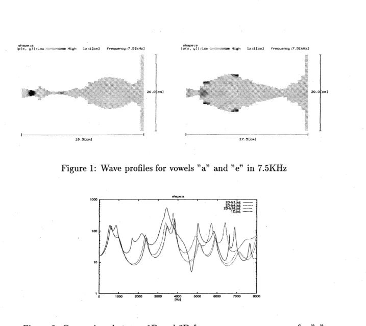
We show a numerical example of $2\mathrm{D}$ wave propagation in the vocal tract open to an

infinite cylinder. The Fig.1 shows a wave profile with$\cdot$

a time frequency 7.5 $\mathrm{k}\mathrm{H}\mathrm{z}$ for the

shapes of vowels ”

$\mathrm{a}$

”

(left) and ”e”(right). The source is placed on the left edge and the

right side is a radiation boundary. The next Fig.

2

shows a frequency response curve for

$,,\mathrm{a}$”measured at the mid point on the radiation boundary. We can see that, as the shape

of the vocal tract becomes flatter, the response curve approaches nearer to the one of 1D

$|\mathrm{p}(\mathrm{X}\mathrm{s}\mathrm{m}.\mathrm{a}9^{)}\mathrm{I}\llcorner_{\circ \mathrm{W}}:.\cdot\cdot.\cdot.\cdot\cdot.\cdot\cdot.\cdot\cdot.\cdot\cdot.\cdot\cdot-\mathrm{H}\mathrm{l}\mathrm{s}h1\mathrm{z}:1\mathrm{R}\mathrm{f}r\epsilon \mathrm{q}-75\mathrm{r}M3$

$\mathrm{s}-\cdot \mathrm{e}$

I$\mathrm{p}\mathrm{t}\mathrm{x}$. $Q’|\mathrm{L}\mathrm{m}..\cdot.\cdot.\cdot\cdot..\cdot.\cdot\cdot..\cdot...\backslash \backslash \backslash \infty \mathrm{H}_{1}\mathrm{g}\mathrm{h}$ $1\mathrm{z}:\iota[\epsilon-1$ $F$requency75$[\mathrm{k}\mathrm{H}_{\mathrm{Z}}]$

Figure 1: Wave profilesfor vowels ”

$\mathrm{a}$” and

”

$\mathrm{e}$

” _in

_7.

$5\mathrm{K}\mathrm{H}\mathrm{z}$

Figure

2:

Comparison between 1D and $2\mathrm{D}$ frequency response

curves

for ”$\mathrm{a}$

”

6

Concluding Remarks

We have developed a methodology to calculate problems in unbounded regions by use of

the $\mathrm{D}\mathrm{t}\mathrm{N}$ mapping or its approximations. Error analysis is given as an extension of the

standard method. Application to a problem having resonance phenomena is presented and

some typical phenomena have been captured inthese

numerical

experiments. Applications

to more realistic problems are future subject of study.

References

[1] Kako, T.

:

Approximation of the scatteringstate by means ofthe radiation boundary

condition, Math. Meth. in the Appl. Sci.,

3

(1981)

506-515.

[2] Mikhlin, S.G.: Variational Methods in Mathematical Physics, Oxford, Pergamon