A Cross-Licensing System Discourages R&D
Investments in Completely Complementary
Technologies
journal or
publication title
Discussion paper series
number
27
page range
1-26
year
2005-09-25
DISCUSSION PAPER SERIES
Discussion paper No.27
A Cross-Licensing System Discourages R&D Investments
in Completely Complementary Technologies
Makoto Okamura Hiroshima University
Tetsuya Shinkai Kwansei Gakuin University
and Satoru Tanaka
Kobe City University of Foreign Studies September 2005
SCHOOL OF ECONOMICS
KWANSEI GAKUIN UNIVERSITY
A Cross-Licensing System Discourages R&D
Investments in Completely Complementary
Technologies
∗
Makoto Okamura
†, Tetsuya Shinkai
‡and Satoru Tanaka
§September 25, 2005
Abstract
We consider the research and development(R&D) investment com-petition of duopolistic firms in completely complementarty technolo-gies. By ”completely complementary technologies,” we mean that no firm can produce the goods without both of the technologies. We derive the investments competiton equilibria in R&D of the two com-pletely complementary technologies with and without a cross-licensing system. By comparing R&D investment levels in the two equilibria, we show that the cross-licensing system discourages the R&D invest-ments when the duopolistic firms produce goods by using the two completely complementary technologies.
Key Words: completely complementary technologies, cross-licensing sys-tem, R&D investments JEL Classification Numbers: D45, L13, O32 A title suggestion for the running head: A Cross-Licensing System in Completely Complementary Technologies
∗We thank Kuninobu Takeda and Sadao Nagaoka for their helpful comments and
sug-gestions on this work. This research was supported by a grant-in-aid from the Zengin Foundation for Studies on Economics and Finance and by Grant-in-Aid (No.14530066) from the MEXT in Japan. Crresponding to: Dr. Tetsuya Shinkai, School of Economics, Uegahara, Nishinomiya, Hyogo 662-8501 JAPAN, E-mail: [email protected], FAX 81-798-510944
†Faculty of Economics, Hiroshima University, Hiroshima JAPAN ‡School of Economics, Kwansei Gakuin University, Hyogo JAPAN §Kobe City University of Foreign Studies, Kobe JAPAN
1
Introduction
In some industries, one feature of recent technological innovation is that the firms cannot produce a commodity without using the outcome of plural distinct inventions. Especially in information technology (IT) industries, one product is comprised of numerous separable patentable elements. For example, the production of a mobile phone having a digital camera involves about 19,000 (Japanese) patents and/or utility models.1 In this environment,
which is named “cumulative-systems technologies” (Merges and Nelson [9]) or “complex technologies” (Cohen, Nelson and Walsh [2]), the inventors of the separable patentable elements tend to be different economic agents. In such cases, the coordination among these inventors affects the interests of each inventor and also affects their R&D incentives. In fact, over the last decade of the previous century, a number of studies discussed the effects of the relationships among inventions on R&D activities, licensining, and the patent systems.
Considering complex technologies, we can identify at least ideally two types of relationships among inventions. The first type is cumulative. In this relationhips, as Scotchmer [13] pointed out, an inventor should engage in R&D activities based on the outcome of preceding inventions. With re-spect to cumulative technological innovations, Green and Scotchmer [5], and Chang [1] showed that externalities due to the lack of coordination among
the creators of plural distinct inventions decreased the incentives of each to invent and develop.
The second type of the relationships among the inventions is complemen-tary. As we typically have seen in the IT industries, technological innova-tions occur on the basis of plural distinct inveninnova-tions developed in different systems of technologies. In this environment, distinct technologies are com-plementary to each other as parts of the product produced. Of course, in complementary technological innovation, an externality problem occurs due to a lack of coordination among the discoverers of plural complementary technologies. Heller and Eisenberg [8] pointed out that the existence of such externality brings a result known as ”the tragedy of anti-commons.” When the intellectual property rights of plural distinct technologies are assigned to different agents (firms), an externality brings excessive exercise of exclusive rights and underutilization of these technologies and discourages incentives for R&D activities of agents(firms).
When all complementary technologies are necessary to produce a prod-uct, cross-licensing has strategic importance. If two different firms own one of two distinct inventions with perfect complementarity, then the two can-not produce a product at all without a cross-licensing contract. In prac-tice, as empirical analyses in the appliance and IC industries conducted by Grindley and Teece [6] and Hall and Ziedonis [7] show, the conditions of the firms’ cross-licensing of products have a great effect on the incentives of each for R&D activities in industries where perfectly complementary inventions
are indispensable for producing the product. In the economics literature, however, few theoretical studies have examined how the conditions of firms’ cross-licensing of technologies affect the firms’ incentives for R&D activi-ties. Fershtman and Kamien [4] offered one of the few studies of such incen-tives. They considered a four-stage model in order to focus on the dynamic prospect of technological innovation. In their model, the first stage involved initial research in which the firms start to develop the two complementary technologies. Once each has succeeded in developing at least one of the two technologies each firm can decide whether to licence–stage 2– or to proceed to stage 3(without licensing) and to continue the innovation race. When at least one of the firms possesses both technologies, either through licensing or through its own development, the game is in stage 4, and the firms produce their goods and interact in the market. However, in reality, the pace of the innovation race of complementary technologies is very rapid and the time horizon is very short in which technologies have economic value in the IT industries. The model setting in which there are two research stages may not be suitable for our analysis.
Hence, in this paper, we will analyze on how a cross-licensing system affects firms’ incentives for R&D activities in a Cournot duoply model in which there are one innovation race stage, one decision-to-license stage and one production competition stage. When one of the firms succeeds in devel-oping both technologies, the market becomes monopolistic since the firm has no incentive to licence its technologies unilaterally to its rival. Note that the
only situation in which licensing may occur is a cross-licensing model when each firm succeeds in developing only one of the distinct technologies. There-fore, in our analysis, we focus on the case in which each duopolistic firm can invest in R&D for both of the two distinct inventions that have strong com-plementarity to each other. We conduct our analysis using a static model with respect to each firm’s R&D investment; we do not examine dynamic aspects of innovation.
In section 2, we describe our model. In section 3, we analyze the problem of R&D under the assumption of Cournot duopoly with completely comple-mentary technological innovations without licensing. In section 4, at first, we examine the conditions under which cross-licensing might occur. Then, extending our analysis to the case with cross-licensing, we examine how the existence of a cross-licensing system affects the firms’ incentives for R&D activities. In the final section, we present our concluding remarks.
2
Model
Let us consider a duopolistic market in which two firms x and y supply a homogeneous product. At the first stage, each firm simultaneously invests in R&D for the two distinct but perfectly complementary technologies, A and B. By “perfectly complementary technologies,” we mean that neither firm can produce the goods without using both of the two technologies. Denote by xA, xB(≥ 0) and yA, yB(≥ 0) the investment levels for technologies A, B of
firm x and the investment levels for technologies A, B of firm y, respectively. When a firm succeeds in the development of both of these technologies or when a firm use the two technologies through licensing, the firm can produce the product. Assume that each firm has constant returns to scale in its production technology and that the marginal and average costs are zero for simplicity. At the end of the first stage, “nature” chooses whether each firm succeeds in the development of the technologies or not. Suppose that each firm succeeds in the development of technology j with probability
p(xj) = 1− e−xj, p(yj) = 1− e−yj, j = A, B. (1)
These probability functions p(·) are well defined since we have, p0(·) > 0, p00(·) < 0, lim
x→0p0(x) =∞, limy→0p0(y) =∞.2
We also assume these functions are identically and independently dis-tributed.
At the beginning of the second stage, each firm knows all successes or failures of both firms’ development efforts with respect to the technologies. At the second stage, if a cross-licensing system is available, each firm bargains
2In this paper, we assume the effect of the R&D activity on the process of
innovation is static. These properties of the success probability function are similar to those of the dynamic “memoryless” or “Poisson” patent race model associated with Reiganum[12]. In her model, the research technology is characterized by the assumption that a firm’s probability of making a discovery and obtaining a patent at a point of time depends only on this firm’s current R&D investment level and not on its past R&D experience. For introductory illustration of the dynamic patent race model, see section 10.2 of chapter 10 in Tirole[14].
with its rival and agrees to a cross-licensing contract, and they divide the total profit according to Nash bargaining. If a cross-licensing system is not available, the game proceeds to the third stage. At the third stage, there are two possible market structures, a monopoly and a duopoly. When only one firm succeeds in the development of the two technologies, this firm is able to be a monopolist and enjoys a monopoly profit, πM. When the two firms
succeed in developing the two technologies, the market structure becomes a duopoly, and each firm earns a duopoly profit πD 3.
Here we assume that4
πM > 2πD. (2)
3
R&D investment without cross-licensing–
—A benchmark
In this section, we introduce as a benchmark the case in which cross-licensing is not available to the firms. After each firm invests in R&D for the two
3As a result of using a static framework, we don’t exclude the possibility of the
simul-taneous success of R&D with respect to technology A and/or B. When the firm can invent around the other patent in technology A(B), the expected profit of each firm in the event of simultaneous success is represented by πD.
4When market demand is linear and each firm has constant returns to scale
technologies during the first stage, nature chooses the outcome of each firm’s investment. Denote the t th outcome by
θt = [XtA, XtB, YtA, YtB] ∈ Θ, where X j t, Y j t ∈ {0, 1}, j = A, B and X j t =
1, Ytj = 0 implies that firm x succeeded in the development of technology j, while firm y failed to develop technology j. Because cross-licensing is not available, we focus on the outcomes in which at least one firm can produce the product. Under these conditions, all meaningful θt s are θ1 = [1, 1, 1, 0],
θ2 = [1, 1, 0, 1], θ3 = [1, 1, 0, 0], θ4 = [1, 1, 1, 1], θ5 = [1, 0, 1, 1], θ6 = [0, 1, 1, 1],
and θ7 = [0, 0, 1, 1]. The outcomes if firm x can produce the goods are three,
in which firm x enjoys a monopoly: θ1 = [1, 1, 1, 0], θ2 = [1, 1, 0, 1],and
θ3 = [1, 1, 0, 0]. The outcome of duopoly is θ4 = [1, 1, 1, 1]. The other
three of these seven outcomes represent the case in which firm y can enjoy a monopoly profit.
The expected profit of firm x, πx(xA, xB, yA, yB) is given by
πx(xA, xB, yA, yB) = (1− e−xA)(1− e−xB)(1− e−yA)(1− e−yB)πD (3)
+(1− e−xA)(1
− e−xB)
{(1 − e−yA)e−yB +
(1− e−yB)e−yA + e−yA
· e−yB
}πM − xA− xB.
M ax πx(xA, xB, yA, yB), given yA, yB.
The first order condition with respect to xA is give by
∂πx ∂xA = e−xA(1 − e−xB)(1 − e−yA)(1 − e−yB)πD +e−xA(1 − e−xB) {(1 − e−yA)e−yB
+ (1− e−yB)e−yA+ e−yA
· e−yB
}πM − 1 = 0. (4)
Since all the probability functions p(·) are identical, we focus our analysis on a symmetric Nash equilibrium. Let us denote the probability of the development of technology by s = e−xA = e−xB = e−yA = e−yB = e−x. The
first-order condition (3) is rewritten to be
s(1− s)3πD + s2(1− s)(2 − s)πM − 1
= s(1− s){(1 − s)2πD + s(2− s)πM} − 1 = 0. (5)
Nash equilibrium if it satisfies the second-order condition. We have ∂2πx ∂x2 A =−e−xA(1 − e−xB)(1 − e−yA)(1 − e−yB)πD −e−xA(1 − e−xB) {(1 − e−yA)e−yB
+(1− e−yB)e−yA + e−yA
· e−yB }πM, (6) and ∂2πx ∂xB∂xA = e−xAe−xB(1 − e−yA)(1 − e−yB)πD +e−xAe−xB {(1 − e−yA)e−yB
+(1− e−yB)e−yA + e−yA
· e−yB
}πM. (7)
Since s∗ satisfies equation (4), we have
¯ ¯ ¯ ¯ ∂2πx ∂x2 A ¯ ¯ ¯ ¯ s=s∗ = −s∗(1− s∗){(1 − s∗)2πD + s∗(2− s∗)πM} = −1, (8)
and ¯ ¯ ¯ ¯ ∂2π x ∂xB∂xA ¯ ¯ ¯ ¯s=s∗ = (s∗)2{(1 − s∗)2πD + s∗(2− s∗)πM} = (s ∗)2 s∗(1− s∗) = s∗ 1− s∗, (9)
where the second equality holds since s∗ satisfies equation (4).
Thus, the second-order condition is given by
¯ ¯ ¯ ¯ ∂2πx ∂x2 A ¯ ¯ ¯ ¯ s=s∗ =−1 < 0, (10) and ¯ ¯ ¯ ¯ ¯ ¯ ¯ ∂2π x ∂x2 A ∂2π x ∂xB∂xA ∂2π x ∂xB∂xA ∂2π x ∂x2 A ¯ ¯ ¯ ¯ ¯ ¯ ¯ s=s∗ = ¯ ¯ ¯ ¯ ¯ ¯ ¯ −1 1−ss∗∗ s∗ 1−s∗ −1 ¯ ¯ ¯ ¯ ¯ ¯ ¯ = 1− µ s∗ 1− s∗ ¶2 > 0 . (11)
We can show that if s∗ satisfies 0≤ s∗ < 12, then inequality (9) holds. Proposition 1 Suppose that πD + 3πM > 16. Then, there exists a sym-metric Nash equilibrium investment level
x∗ =− ln s∗
L >− ln( 1 2)
When there is R&D investment competition in an industry with completely complementary technologies without a licensing system.
Proof. Let the left-hand side of equation(4) equal φ(s), then φ(s) can be
rewritten into
φ(s) = [πM − πD]s4− 3[πM − πD]s3+ [2πM − 3πD]s2+ πDs− 1. (12)
From the assumption, πM
− πD > πM
− 2πD > 0, we have
lim
s→+∞φ(s) = lims→−∞φ(s) =∞. (13)
Furthermore, from (10) and the assumption of this proposition, we see that φ(0) = φ(1) =−1 < 0 and φ(1/2) = π D+ 3πM 16 − 1 > 0. (14) Also we have φ0(s) = (1− s)2(1 − 4s)πD + s(4s2 − 9s + 4)πM, so φ0(0) = πD > 0 and φ0(1) =−πM < 0. (15)
s ∈ [0, 1] such that φ0(s) = 0.
Now, let λ1, λ2 and λ3 be the three roots of equation φ0(s) = 0. We have
(s−λ1)(s−λ2)(s−λ3) = s3−(λ1+λ2+λ3)s2+(λ1λ2+λ2λ3+λ3λ1)s−λ1λ2λ3 = 0. (16) Dividing φ0(s) = 4[πM − πD]s3 − 9[πM − πD]s2+ 2[2πM − 3πD]s + πD = 0 by 4[πM − πD], we get s3− 9 4s 2+ 2πM − 3πD 2[πM − πD]s + πD 4[πM − πD] = 0. (17)
By comparing (14) and (15), we obtain
λ1+ λ2+ λ3 = 9 4 > 0, (18) λ1λ2+ λ2λ3+ λ3λ1 = 2πM − 3πD 2[πM − πD], (19) and λ1λ2λ3 =− πD 4[πM − πD] < 0. (20)
roots are negative , (ii)two roots are positive and one root is negative, or (iii)two roots are imaginary and one root is negative. However, from (11), (12), and (13), we see that cases (i) and (iii) never occur, and we can see therefore conclude that case (ii) occurs. Here, suppose that 0 < λ1, λ2 < 1,
and λ3 < 0. Then, λ1+ λ2+ λ3 < λ1+ λ2 < 2 holds, but if so, this conclusion
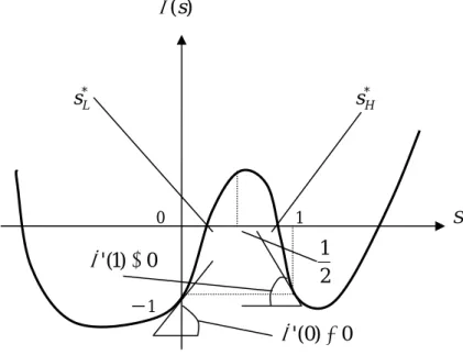
and (16) contradict each other. Thus we have one negative root, one positive root in {s : 0 < s < 1} , and one positive root in {s : s > 1}. In addition to this argument and the fact that φ(s), the biquadratic function of s, has at most three extreme points, we can conclude that φ(s) is unimodal in s∈ [0, 1] , so it has a maximum point as shown by Figure 1. Therefore we have two s∗ ∈ (0, 1) , say s∗L and s∗H such that 0 < s∗L < 12 < s∗H < 1. However, we see that only s∗
L (< 12) satisfies the second-order condition (9), and the result
follows.
[Insert Figure 1 here]
4
R&D investment with cross-licensing
In this section, we investigate the case in which firms(a firm) can license to each other their (its) technology (technologies) if they(it) succeed(s) in the development of the technology(technologies). We assume that they determine a licensing fee by Nash bargaining if they agree to have a licensing contract. We assume that after the licensing agreement each firm produces
Cournot equilibrium quantity of output under the realized marginal cost incurred with benefit of licensing.5
We can see two possible cases in which licensing may occur. From the assumptions about the symmetry of the firms, we can focus on the cases in which firm x licenses its technology to firm y. In θ3 = [1, 1, 0, 0], the market
becomes a monopoly controlled by firm x , so it has no incentive to license its technologies to its rival.
(Case 1) θ1 = [1, 1, 1, 0] or θ2 = [1, 1, 0, 1]
In this case, unilateral licensing of one technology may occur from firm x to firm y. Consequently, the market becomes a duopoly. Denoting the
license fee by N1 , the Nash bargaining function B1 is given by
B1 = [πD+ N1− πM][πD− N1].
5Both firms may agree to a contract in which a licensee firm is obligated to pay to the
licensor firm half of the monopoly profit brought by producing at the lowered marginal cost realized by the licensing; the license fee would serve as compensation for no production of the good by the licensor. The final gain of each firm after the payment of this contract is, of course, larger than that realized when firms compete in a Cournot manner as we assumed in our model. However, the former is interpreted as an illegal act from the antitrust point of view. See the discription in Section 3.2 and Example 4 in the Appendix of “Antitrust Guidelines for Collaborations among Competitors [3]” issued by the U.S. Federal Trade Commission and the U.S. Department of Justice. They say that “Agreements of a type that always tends to raise price or reduce output are per se illegal.” Thus a contract under which only the licensee produces the monopoly output and pays half of the monopoly profit as a licensing fee to the licensor seems to be per se illegal. We thank Kuninobu Takeda, associtate professor of Antitrust Law at Osaka University for this suggestion regarding antitrust and for the source of this citation. Hence, we assume that two firms compete in a Cournot manner after the licensing contract.
Then we have ∂B1 ∂N1 = πD − N1− (πD + N1− πM) = πM − 2N1 = 0 or equivalently N1 = πM 2 . The resulting profits of firm x and firm y are
πD+ π M 2 , π D − π M 2 ,
respectively. Since the threat points of firm x and firm y are πMand 0, respectively, these profits are greater than the profits of firms x and y after side payment for licensing. So licensing may not occur in this case.
(Case 2) θ8 = [1, 0, 0, 1] or θ9 = [0, 1, 1, 0].
In these cases, cross-licensing between firm x and firm y occurs, and the market becomes a duopoly. Denote by N2 the license fee, the Nash
bargaining function B2 is given by
B2 = [πD+ N2][πD− N2].
Then we have
∂B1
∂N1
or equivalently
N2 = 0.
The profits of firm x and firm y after side payment for licensing are identical,
πD,
which is greater than the threat-point profit, zero. Cross-licensing occurs. From the above observation, the expected profit of firm x with cross-licensing, f πx(xA, xB, yA, yB) is given by f πx(xA, xB, yA, yB) = πx(xA, xB, yA, yB) + (1− e−xA)e−xB·e−yA(1 − e−yB)πD + e−xA(1 − e−xB)(1 − e−yA)e−yBπD. (21)
Note that the second (third) term of (21) shows an additional expected profit associated with the cross-licensing contract if firm x succeeds in the development of technology A (B), while firm y succeeds in the development of tehnology B(A). By using symmetry, the profit-maximizing condition with respect to xA can be written as
∂fπx ∂xA = ∂πx ∂xA + e−xAe−xBe−yA(1 − e−yB)πD − e−xA(1 − e−xB)(1 − e−yA)e−yBπD = φ(s) + s2(1− s)(2s − 1)πD = 0. (22) Define ψ(s)≡ φ(s) + s2(1− s)(2s − 1)πD = φ(s) + (−2s4+ 3s3− s2)πD. (23) Then, we have ψ(0) = φ(0) = ψ(1) = φ(1) =−1. (24) Since ψ0(s) = φ0(s) + s(−8s2 + 9s− 2)πD, (25) we get ψ0(0) = φ0(0) = πD > 0 (26)
and
ψ0(1) = φ0(1)− πD =−πM − πD < φ0(1) =−πM < 0. (27)
Rearranging ψ(s)with respect to s yeilds
ψ(s) = [πM − 3πD]s4− 3[πM − 2πD]s3+ 2[πM − 2πD]s2+ πDs− 1. (28)
We obtain the following lemma on the extreme points of ψ(s).
Lemma 1 ψ(s) has a unique maximum in [0, 1].
Proof. In order to examine the extreme points of ψ(s),the first-order condi-tion is
ψ0(s) = 4[πM − 3πD]s3− 9[πM − 2πD]s2+ 4[πM − 2πD]s + πD = 0. (29)
Suppose that πM−3πD 6= 0. Then, dividing both sides of (27) by 4[πM−3πD] yields s3− 9[π M − 2πD] 4[πM − 3πD]s 2+ [πM − 2πD] [πM − 3πD]s + πD 4[πM − 3πD] = 0.
Using the relationships between the roots of the cubic equation and coeffi-cients, we have
λ1+ λ2+ λ3 =
9[πM
− 2πD]
λ1λ2λ3 =−
πD
4[πM − 3πD]. (31)
If πM − 3πD < 0, then we see that the right hand sides of (29) and (30) are negative and positive, respectively. If all of the three roots of (27) are real roots, then two of them are negative and one is positive. If (27) has one real root and two imaginary roots, the real root must be positive since (30) has a positive sign. In both cases, (27) has a unique positive real root. Taking this fact and equations (24) and (25) into consideration, we can see that the maximum exists in [0, 1]. Next suppose that πM
− 3πD > 0. In
this case, we see that the right-hand sides of (29) and (30) are positive and negative, respectively. Since the sign of (30) is negative, as we see on φ(s) in the proof of proposition 1, we can see that any of the following three cases holds: (i) all roots are negative, (ii) two roots are positive and one root is negative,or (iii) two roots are imaginary and one is negative. However, from the signs of (29)and (30), we see that cases (i) and (iii) never occur. So we can conclude that case (ii) occurs. Here suppose that 0 < λ1, λ2 < 1
and λ3 < 0. Then, λ1 + λ2 + λ3 < λ1 + λ2 < 2 < 94 < 9[π
M
−2πD] 4[πM−3πD]holds,
since πM − 3πD > 0. But then this and the fact that the sign of (29) is positive contradict each other. So (27) must have one negative root, one positive root in {s : 0 < s < 1} and one positive root in {s : s > 1}. From this fact and (24), (25), we can see that there exists a maximum in [0, 1]. Finally suppose that πM
− 3πD = 0. Then, from (26) we have
ψ(s) =−3[πM
− 2πD]s3+ 2[πM
− 2πD]s2 + πDs
+πDs
− 1. So we also have ψ0(s) =−9πDs2+ 4πDs + πD = 0. Dividing
both sides of this by πD(
6= 0) yields: −9s2 + 4s + 1 = 0. Solving this with
respect to s, we get
s∗ = 2± √
13
9 .
So ψ(s) has a unique maximum s∗ = 2+√13
9 in [0, 1]. It has a maximum point
as shown by Figure 2, and the lemma holds.
[Insert Figure 2 here]
¿From (21), we can easily show that
ψ(s)S φ(s) ⇔ s S 1
2. (32)
Combining (22), (23), (24), and (25) with Lemma 1, we can present our main result.
Proposition 2 Suppose that πD + 3πM > 16. Then, there exists a
sym-metric Nash equilibrium investment level xe∗
x∗ =− ln s∗
L >xe∗ =− ln es∗L>− ln( 1 2)
in R&D investment competition with completely complementary technolo-gies with a licensing system.
Proposition 2 above states that the introduction of a cross-licensing sys-tem discourages each firm’s R&D investment, when duopolistic firms can produce goods by using two completely complementary technologies. Let
us explain an economic intuition behind this result. Consider that firm x increases infinitismaly its R&D investment for the technology A. The cross-licensing system adds two terms to the expected profit of each firm without cross-licensing, shown in (21). The second and third terms in (22) indicate the marginal revenue associated with the introduction of the cross-licensing system. The R&D investment increases the success probability of the tech-nology A’s development and raises the expected profit resulting from licensing the technology A to firm y. This positive effect appears in the second term in (22). On the other hand, this R&D investment reduces the failure prob-ability of the technology A’s development, or the probprob-ability that firm x can introduce the technology A from firm y in exchange of its developed tech-nology B. This generates a unfavorable impact on the expected profit shown in the third term of (22). This negaive effect shows an opportunity cost associated with the R&D investment. The equilibrium level of R&D invest-ment without a cross-licensing system is sufficiently high and the resulting success probability of development is also high (it exceeds 1/2). Since this initial R&D investment is high, the marginal opportunity cost dominates the marginal benefit (revenue), if each firm engages in the coss-licensing system and increases its R&D investment. Each firm, then, has an incentive to decrease its R&D investment.
5
Concluding Remarks
In this paper, we have explored by analyzing a simple static innovation model the incentives for R&D investment by duopolistic firms facing technological innovation in completely complementary technologies. At first, as a bench-mark we derived the symmetric Nash equilibrium investment levels in R&D between competing firms in completely complementary technologies without a licensing system. We examined the conditions under which cross-licensing occurs. Then, by deriving the symmetric Nash equilibrium investment levels of this model, we investigated how the existence of a cross-licensing system affects firms’ incentives for R&D activities in a Cournot duopoly. We also showed that the existence of a cross-licensing system discourages a firm’s R&D investments. Intuitively, we would suggest that the existence of a cross-licensing system decreases the firms’ incentives for R&D through the chance that they may each benefit from the exchange of their technologies.
There remain many topics for future research. We focused on the sym-metric equilibrium in order to make our analysis easy. In reality, however, firms cannot be symmetric in industries where complementary technologies are indispensable for the production of goods. The role of R&D ventures that do not produce products but concentrate on R&D, increases in prominence in such industries. Also, since we concentrated on the effect on incentives for R&D, we did not examine the effects on social welfare at the equilibrium. To clarify how governments should plan and exercise policy for
technolo-gies under complementary technological innovations, it is important for us to explore the implications on economic welfare at the equilibrium in our model.
References
[1] Chang, H. F. (1995), “Patent Scope, Antitrust Policy, and Cumulative Innovation,” Rand Journal of Economics, vol. 26: pp. 34-57.
[2] Cohen, W. M., R. R.Nelson and & J. P. Walsh. (2000), “Protecting Their Intellectual Assets: Appropriability Conditions and Why U.S. Manufac-turing Firms Patent (or Not),” NBER Working Paper, No. 7552. [3] Federal Trade Commission and the U.S. Department of Justice
(2000), Antitrust Guidelines for Collaborations among Competitors, http://www.ftc.gov/os/2000/04/ftcguidelines.pdf.
[4] Fershtman, C., and M. I. Kamien. (1992), ”Cross Licensing of Com-plementary Technologies,” International Journal of Industrial Organi-zation, vol. 10: pp. 329-48.
[5] Green, J. R., and S. Scotchmer. (1995), “On the Division of Profit in Sequential Innovation,” Rand Journal of Economics, vol. 26: pp. 20-33.
[6] Grindley, P. C. , and D. J. Teece. (1997), “Managing Intellectual Capi-tal: Lisensing and Cross-Licensing in Semiconductors and Electronics,” California Management Review, vol. 39: pp. 8-41.
[7] Hall, B. H.,and R. H. Ziedonis. (2001), “The Patent Paradox Revisited: An Empirical Study of Patenting in the US Semiconductor Industry, 1979-1995,” Rand Journal of Economics, vol. 32: pp. 101-428.
[8] Heller, M. A.,and R. S. Eisenberg. (1998), ”Can Patents Deter Innova-tion? The Anticommons in Biomedial Research,” Science, vol. 280: pp. 698-701.
[9] Merges, R. P., and R. R. Nelson. (1994), “On Limiting or Encouraging Rivalry in Technical Progress: The Effect of Patent Scope Decisions,” Journal of Economic Behavior and Organization, vol. 25: pp. 1-24. [10] Nihon Keizai Shinbun (18 August 2003)
[11] Okamura, M., T. Shinkai., and & S. Tanaka. (2002),“A Cross-licensing System Discourages R&D Investments in Completely Complementary Technologies,” Working Paper, Kobe City University of Foreign Studies, no. 14.
[12] Reinganum, J. (1982), “A Dynamic Game of R&D: Patent Protection and Competitive Behaviour,” Econometrica, vol. 50: pp. 671-88.
[13] Scotchmer, S. (1991), ”Standing on the Shoulders of Giants: Cumulative Research and the Patent Law,” Journal of Economic Perspectives, vol. 5: pp. 29-41.
[14] Tirole, J. (1988), The Theory of Industrial Organization, MIT Press, Cambridge.
φ
(s) * L s s*H 0 1 Sφ
'(1)<0 2 1 −1φ
'(0)>0Figure 1 Equilibrium without a cross licensing
φ
(s),ϕ
(s) * s s~ϕ
(s)Figure 2 Equilibriums with and without a cross licensing
2 1 s ) ( s φ 1 −