Efficient Autocompletion with Error Tolerance

(1)

DEIM Forum 2016 D4-1

Efficient Autocompletion with Error tolerance

Sheng HU

†

Chuan XIAO

‡

and Yoshiharu ISHIKAWA

†

†Graduate School of Information Science, Nagoya University, Furo-cho, Chikusa-ku, Nagoya, 466-8601 Japan

‡Institute for Advanced Research, Nagoya University, Furo-cho, Chikusa-ku, Nagoya, 466-8601 Japan

E-mail: †[email protected], ‡{chuanx, y-ishikawa}@nagoya-u.ac.jp

Abstract Most popular search engines have provided query autocompletion features in their systems. When a user issues a query, without inputting complete keywords, the search engine will prompt several options which complete the remaining part of the query automatically. This research will focus on investigating novel techniques for error-tolerant query autocompletion by addressing several key issues of this feature, and eventually improve the efficiency and the accuracy of the query processing. In our work, we proposed an improve expansion algorithm based on current state-of-the-art work. Moreover, we also improve the index reduction method to reduce the index size as much as possible. Experiment results show that our new method can improve the algorithm efficiency and reduce the index size very well.

Keyword Query Autocompletion，Query Processing，Textual Database

1. Introduction

Recently, the user experience of search engine becomes more and more important. Most popular search engines have provided query autocompletion features in their sys-tems. When a user issues a query, without inputting com-plete keywords, the search engine will prompt several op-tions which complete the remaining part of the query au-tomatically.

Moreover, search engines like Google, hav e equipped their system with an advanced autocompletion technique, which is called autocompletion with error tolerance. Even a user issues an uncompleted query which may contain typos, the search engine can still identify the intended query and give the co rrect answers. As more and more users are using smartphones as search engine interface, this feature is considered of great importance and pro-spective.

This research will focus on investigating novel tech-niques for error-tolerant query autocompletion by ad-dressing several key issues of this feature, e.g., improving the efficiency and the accuracy of query processing. Fig-ure.1 shows an example of the result of autocompletion with inputting “coff”.

Figure 1. An example of autocompletion of “coff”

2. Related Work

There are various ways to implement the autocomple-tion technique[1][6]. Currently, trie index[2] becomes very popular and is adopted as the most efficient way among the current research works. The ICPAN algorithm put forward by Guoliang Li [3] is considered the most re-liable trie traversal algorithm while IncNGTrie which is put forward by Chuan Xiao[4] is considered the most ef-ficient trie traversal algorithm. The ICPAN [3] gives a definition about the Pivotal Active Node which is seemed as the basic composition unit of the trie index and can support 2-length characters error tolerance which means the search system can give the correct answer despite of two characters typos. The IncNGTrie[4] uses the Neighbor Generation method[5] so as to include the possibility of typos in advance. In the experiment, it can support 3-length characters error and achieves up to two orders of magnitude speedup over Li’s ICPAN method. However, IncNGTrie achieves the efficiency at the price of sacri-ficing large memory space, and under the special circum-stances the overhead of the space may be unaffordable.

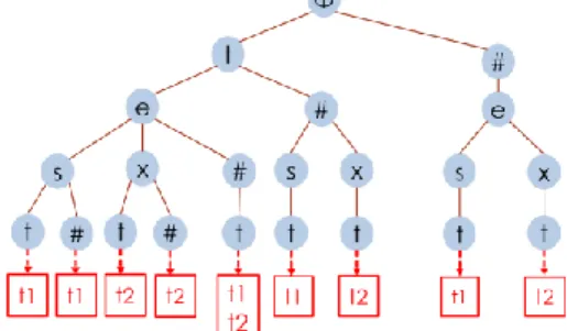
Figure 2. An example of IncNGTrie with keyw ord {test, text} with τ=1

(2)

Example 2 Figure 2. shows a simple example of IncNTrie

Index Structure which consists of two strings t1 and t2. T1 represents “test” and t2 represents “text”. Single path from the root to one leaf represent s one string. For example, from left side, we have Φ-t-e-s-t path, which represents string “test”. Meanwhile we use ‘#’ as the placeholder to represent the deletion conducted on the data string side. Below we give the definition of ‘#’.

Definition 1 (Placeholder ‘ #’) We use ‘#’ to create more

deletion-marked variant[7,8] , that is, ‘#’ means at this

position one character is deleted from a data string. E.g., “ts”, a 2-variant of “test”, will be represented as “t#s#”. Meanwhile, we will generate all the 1-variant of “test”, which is {#est, t#st, te#t, tes#}. And finally use these variants to construct the trie as Figure 2. shows. Moreover, we use τ as the threshold to limit the error -tolerant ability of this index.

3. Index reduction

As IncNGTrie has the shortcoming of space cost, I be-gan my work from reducing the space of IncNGTrie, I also propose a new expansion algorithm of the trie traversal algorithm to improve the traversal efficiency. After that, I’m doing the work of result ranking to improve the qual-ity of results as much as possible.

In IncNGTrie research, they used two techniques to re-duce the index size as much as possible, so as to make it fit the computer memory. One is Common Data String Merge, the other is Common Subtree Merge. After my experiments, I found some disadvantages of these two techniques. For the former one, this work simply does the reduction exhaustedly without any consideration of the reduction extent parameterization. Thus I come up with the idea that I can introduce the parameter p to control the reduction extent. In the original work, this parameter is set to 1, that is, only when the parent node share completely the identical data strings, it’ll be merge into 1 string, which drastically limits the benefit of the reduction. And after I introduce this parameter BRC, we can generally control the benefit and gain from the common data string merge technique. Here we give the definition of Branch Reduction Control.

Definition 2 BRC (Branch Reduction Control)

We use BRC as the parameter to control how much we will reduce the index size. First we will traverse the whole trie in a Depth-First order, and check every nodes to see if its descendants amount is lower than BRC, if so, we will

prune all the path which contain ‘#’ in the subtree from current node.

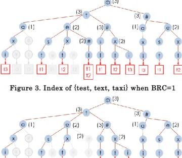
Example 3 Figure 3, Figure 4, Figure 5 give an example

of the trie variation under the condition when we increase BRC from 1 to 3 consecutively. If we set the BRC param-eter to 1, the leaf nodes’ parent node will be merged when the descendant identical data string number less equal s than 1. Numbers in the bracket represent the amount of the descendant identical data string under each node. As showed in Figure 3, note that in the left subtree under the node “a”, as all the descendants under “a” only represent the same string “t3”, all the paths start from “a” and con-tain “#” will be removed from the index. In Figure 3, we change the nodes’ color into grey if they are removed. In Figure 4 and Figure 5, we increase BRC to 2 and 3, as the nodes satisfying our reduction condition increase quite a lot, we can find the index size will be reduced incremen-tally. Especially when BRC=3, we successfully prune al-most a half part in our example. In our experiment, this change will reduce the size of our tree drastically when τ is larger than 1 and decrease a little bit on the search time side because this is an inevit able tradeoff between the storage and efficiency. Moreover, I change the underlying data storage to make all the identical data point to just one copy instead of store a copy for every redundant record. The parameter we introduce could be adjusted accordin g to the requirement of the real environment.

Figure 3. Index of {test, text, taxi} when BRC=1

(3)

Figure 5. Index of {test, text, taxi} when BRC=3

4. Expansion algorithm improvement

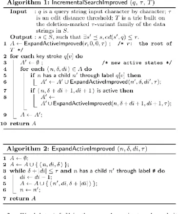
To support the active node model proposed in Li’s paper, Xiao’s work used a triplet <node, cursor, incoordination> as the representation of the active node states . This makes the expansion algorithm much more tedious and it gener-ate too many active nodes s tgener-ates which consume quite a lot resources of the memory. To fix this problem, I change the active node representation to <node, incoordination, dif-ference in trailing’#’>, which simplifies the model dras-tically and generate much less active node states dur ing the expansion procedure. Our experiment shows that compared with the original work, the intermediate active nodes number is reduced by over 50%. Moreover, I also change the BST method to remove the second duplicate data because the original lemma suppo rting the old method is not reliable.

To search an index constructed like Figure 2, we need traverse the trie with the single stroke of query input. In Li’s work, <node, incoordination> is used to represent the active node state because the index construct ed is a direct trie. In Xiao’s work, <node, cu rsor, incoordination> is used instead because its new index structure IncNGTrie. Now we adjust it into <node, incoordination, difference> and give the explanation based on Xiao’s work.

In line 1 of Algorithm1, we use ExpandActiveImproved to initialize the original active states. At this moment, there’s no query stroke is input. τ represents the threshold of error’s upper bound, we first go through the trie from root to most τ #’s and set the corresponding node to active. And then from line 2, we can see user will input a query stroke q[v], with the new stroke, algorithm will expand new active states based on original ones. Line 4 to line 9 shows the method. When a query stroke q[v] comes, for each active state <node, incoordination, difference>, we do two steps:

1. We keep ‘q[v]’ in the query’s variant, so we’ll go through ‘q[v]’, and then go through ‘#’ in the trie.

2. We delete ‘q[v]’ in the query’s variant and mark it as ‘#’. So we’ll see if current node is still active by checking incoordination and difference, and then go through ‘#’ in the trie.

After processing all the query strokes, the final set A is returned and used to fetch the results .

5. Experiment

The experiments were implemented using a PC with Intel Core i5 CPU (2.60GHz), 4GB memory, and Windows 7 OS. The dataset was made by extracting the string of POI of the GNIS dataset. This dataset consists of 200400 strings and average string length is 11.

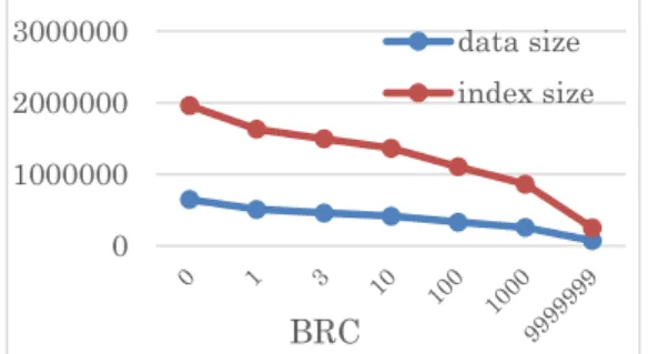
5.1 Effect of index reduction

We first evaluated the effect of our index reduction method. Figure 6, Figure 7, Figure 8 corresponds to the situation when τ=1, 2 and 3. The value of τ represents the error-length, that is, how many errors the query can con-tain at most. Y-axis represents the amount of data strings and index nodes. Here, we use data size to represent the data strings amount. Because we merge the subtree’s node and its leaf nodes, some identical data strings we store in the memory will be merged into one. Then, we use index size to represent the index nodes amount. From the ex-periments, we can see that when BRC variates from 0 to 1, both data size and index size is reduced by almost 30%,

(4)

and the larger tau is, the more the total size is reduced. When BRC is increased to 9999999, the whole IncNGTrie is degenerated to a direct trie, which has a very small size.

Figure 6. Data size and index size reduction effect when τ=1

5.2 Effect of expansion improvement

Figure 9. Returned active nodes amount when τ=1 The three figures Figure 9, Figure 10, Figure 11 show the expansion improvement effect under the condition τ=1, 2 and 3. X-axis represents the query length and Y-axis represents the active node states amount. The common point of the three is that, as the length of query word

in-creases, the improved expansion algorithm has much less active states, which can remarkably save the memory and improve the time efficiency compared with the old rithm. When query length equals 8, the improved algo-rithm’s active nodes states number is almost a half of the old one, which means our method reduce over 50% active node states when quer y is long enough.

Figure 10. Returned active nodes amount when τ=2

Figure 11. Returned active nodes amount when τ=3

References

[1] L. Boytsov. Indexing methods for approximate dic-tionary searching: Comparative analysis. ACM Jour-nal of Experimental Algorithmics, 16(1), 2011. [2] D. Deng, G. Li, and J. Feng. An efficient trie -based

method for approximate entity extraction with ed-it-distance constraints. In ICDE, pages 762 -773, 2012.

[3] G. Li, S. Ji, C. Li, J. Feng. Efficient Fuzzy Full -text Type-ahead Search. VLDB Journal, 2011.

[4] C. Xiao, J. Qin, W. Wang, Y. Ishikawa, K. Tsuda, K. Sadakane. Efficient Error-tolerant Query Autocom-pletion. Proceedings of the VLDB Endowment, Vol. 6, No. 6, 2013.

[5] T. Bocek, E. Hunt, and B. Stiller. Fast Similarity Search in Large Dictionaries. Technical Report ifi-2007.02, Department of Informatics, University of Zurich, April 2007.

[6] Inci Cetindil, Jamshid Esmaelnezhad, Taewoo Kim, and Chen Li. Efficient instantfuzzy search with proximity ranking. In Data Engineering (ICDE), 2014 IEEE 30t h_{International Conference on, pages 328 –}

339. IEEE, 2014.

[7] Thomas Bocek, Ela Hunt, Burkhard Stiller, and Fabio Hecht. Fast similarity search in large dictionaries. University of Zurich, 2007.

[8] Moshe Mor and Aviezri S. Fraenkel. A hash code method for detecting and correcting spelling errors. Communications of the ACM, 25(12):935 –938, 1982. 0 1000000 2000000 3000000 BRC data size index size 0 5000000 10000000 BRC data size index size 0 5000000 10000000 15000000 20000000 25000000 BRC data size index size 0 10 20 30 old improved 0 100 200 300 old improved 0 500 1000 1500 2000 old improved