PARALLEL COMPUTATION OF COMPRESSIBLE MULTI-FLUID FLOW (Analysis and Numerical Simulation of Complex Fluid Flow)

PARALLEL COMPUTATION OF COMPRESSIBLE MULTI-FLUID FLOW Angel M. Bethancourt L.

Institute ofComputational Fluid Dynamics Masahiro Egami

Honda R&D, Co. Ltd.

Abstract. A collapse ofa helium bubble due to its interactions with an incoming shock

wave

is numerically examined. The flow is modeled using the two-dimensional compressible Euler equations with an additional equation of motion for the propagating interface. The solution is obtained inatwo-step manner, first, the Euler’s system ofequations is solved using Roe’s flux difference splitting scheme; second, the moving interface (a

ffinction ofthe specific heat ratio is used to mark the fluids interface) is captured using

a

third-order WENO scheme. For both, a third-order Runge-Kutta method is used for time integration. The solver is parallelized, allowing

us

to conduct fme mesh computations, and enabling the numerical reproduction of the mechanisms observed in previous published experiments.

1. Introduction

Early attempts to compute multi-fluid flow, consisted in incorporating

a

conservativeform ofthe advection equation for the material interface into the Euler system of equation [1,2,3],

and solve them using standard methods developed for the classical Euler equations.

However, it

was

observed that spurious oscillations develop at the material interfaces due to

differences in fluid propertiesat the interface,

as

wellas,

errors

in the locationofthe interface. In orderto solve

some

ofthe problems,

a

quasi-conservative is proposed in [1], in which the advection equation is decoupled $\theta om$ the Euler equations and written in non-conservative

form.

Additional modifications to the goveming equations are made in [4,5], which render the algorithm “single-fluid” when calculating the interface fluxes at the expense of conservation, to improve the coupling of the advection-Euler equations and to account for

pressure

equilibrium

across

the interface.

Inthis paper, the quasi-conservative method described in [1,4] is implemented. Because our interest is

on

high-resolution computations, this implementation is extended using MPI

(Message Passing Interface) libraries for its parallelization. As application, the

interactions

2. Equationsofmotion

For the problem at hand,

we

limit

our

analysis to two immiscible ideal gases, $p=(\gamma-1)p$ , characterized by their constant ratio of specific heats, $\gamma$

.

The

two-dimensional Euler equations for such multi-component flowin conservative form

are

$\frac{\partial Q}{\partial t}+\frac{\partial E}{\ }+ \frac{\partial F}{\partial y}=0$, (1)

$Q=\{\begin{array}{l}\rho\rho u\rho ve\end{array}\};E=\{\begin{array}{l}\rho upu^{2}+p\rho uv(e+p)u\end{array}\};F=\{\begin{array}{l}\rho v\rho uv\rho v^{2}+p(e+p)v\end{array}\}$

where $p$ isthe density, $u$ and $v$

are

thevelocity components,$p$ isthepressure, and$e$ is the total

energy ofthe fluid.

The moving interface is captured usingthe discontinuity in the ratio of the specific heats for the different components. Since material interfaces

are

advected by the flow, any hnctionof $\gamma$ obeys the advectionequation [1],

$\frac{\partial f(\gamma)}{\partial t}+u\frac{\partial f(\gamma)}{\ }+v \frac{\partial f(\gamma)}{\Phi}=0$,

.

$\cdot$

.

$f( \gamma)=\frac{1}{\gamma-1}$ (2)

Spatial discretization of (1) is done using Roe’s flux difference splitting scheme. The numerical fluxis givenby:

$E_{i+1/2}=E(Q_{L},Q_{R})= \frac{1}{2}[E(Q_{L})+E(Q_{R})]-\frac{1}{2}|A|[Q_{R}-Q_{L}]$, where$A= \frac{\partial E}{\partial Q}$ (3)

$A$ isthe Jacobian matrixbased

on

Roe’s average of$Q_{L}$ and $Q_{R}$

.

The modification introduced

in [4] consists in calculating two fluxes at the cell interface, by “freezing” the values of$\gamma$ in

either side ofthe interface:

$E_{i+1/2}^{L}=E(Q_{L},Q_{R};\gamma_{L})$

$E_{i+1/2}^{R}=E(Q_{L},Q_{R};\gamma_{R})$

Then,

use

$E_{i+1/2}^{L}$to update the flux in cell $i$and $E_{i+1/2}^{R}$to update the flux incell $i+l$

.

The spatial discretization of(2) is carried out using

a

third-order WENO scheme [6]. A TVDthird order Runge-Kutta method is used to solve both the Euler and advectionequations

[6]. The equations

are

written as, $Q_{t}=L(u)$, where $L(u)$ is the discretization of the spatial

$Q^{(1)}=Q^{n}+\Delta tL(Q^{n})$

$Q^{(2)}= \frac{3}{4}Q^{n}+\frac{1}{4}Q^{(1)}+\frac{1}{4}\Delta tL(Q^{(1)})$

$Q^{n+1}= \frac{1}{3}Q^{n}+\frac{2}{3}Q^{(2)}+\frac{2}{3}\Delta tL(Q^{(2)})$

(4)

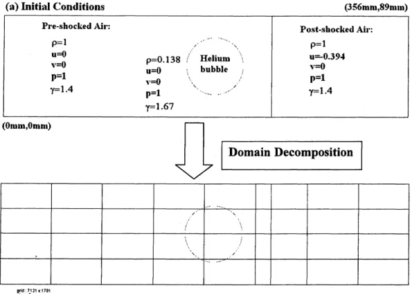
The parallelization of the code is achieved by using Domain Decomposition in conjunction with a SPMD(Single Program Multiple Data)technique. The MPI libraries

are

usedto communicate betweenthe differentprocessors. Our system consists of 8 nodes, each nodecontains of$2cpu$-IntelXeon (8 cores). Themaximum number ofcores available is 64. 3. Problem Definition

Our focusis

on

the dynamics ofthe interaction ofa Mach 1.22 shockand

a

heliumbubble,

as

presented in [7,8]. The initial conditions for this problem

are

given in Fig. 1, the upper and lower boundaries

are

considered solid walls, the inflow is $fi\cdot om$ the right and properties

are

specified, at outflow (left)

a zero

gradient is imposed. A uniform grid with spatial resolution of 0.05

mm

is used for the present computation, resulting in a grid size of 712lxl781. It takes approximately $12 hr30\min$ to obtain a 528 ps sample (time step:

$3.3333x10^{-8}s)$using 32 processors.

4. Computational Results

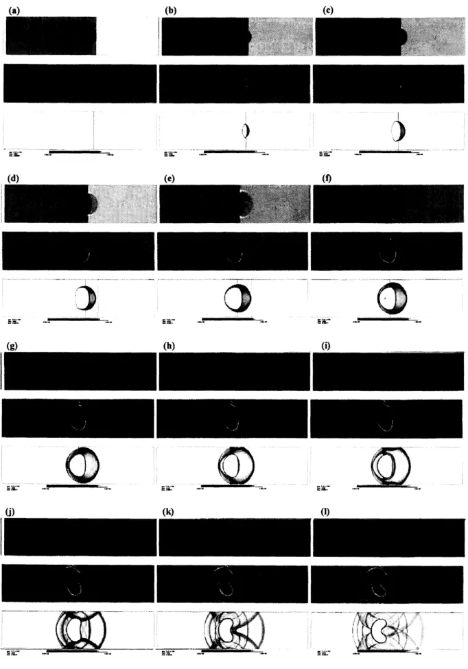
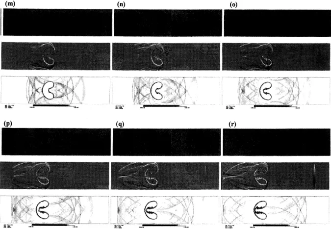
Figure 2 shows a sequence of idealized Schlieren images [8], showing the overall

wave

stmcture. At 24 ps, Figure $2a$ shows

a

reffacted shock inside ofthe bubble, moving faster

than incident shock, since thehelium has ahigher sound speedthan the air. Upstream ofthe bubble, areflected

wave

is shown moving away $\theta om$the bubble. At36 ps, Figure $2b$shows

a

four-shockconfigurationwhich it isusuallytermedtwinregular reflection-reffaction(TRR),

also shown in Figure 3. At 48 ps, Figure $2c$ shows the

re

$\theta acted$

wave

emerging $\theta om$ the

bubble and becoming the transmitted wave, also two cusps appear in the left-side of the bubble indicating intemally reflected

waves

that converge toward the axis of the bubble

(Figure $2d,$ $56$ ps). At 64 ps, Figure $2e$ shows the intemal reflected

waves

diverging after

crossing, and the two branches ofthe transmitted shock

cross

downstream ofthebubble. At 88 ps, Figure 2fthe initial reflected shock has reflected from theupperand bottom walls. At larger times (228 ps), Figures $2g$ shows that the bubble has ffirther deformed into

a

kidney

shaped object. Finally, Figures $2h$ and $2i$ show

an

induced jet of

air

along the axis of the

bubble, resulting inthedevelopment oftwo vorticalstructures.

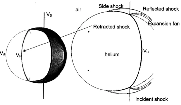
Figure 3 shows the enlargement of the twin regular reflection-refraction (TRR) shock configuration

as

well

as

the locations used to compare the shock

waves

velocities. Table 1

shows the comparison of the present computation

wave

velocities with the experiment of Hass and Sturtevant [7] and Quick and Kami [8] computation. Overall agreement is

excellent, except for the values of the reflected and upstream velocities; this disagreement is due to the existence of bubble contamination which affects the values of its physical properties.

Figure 4

uses

the density, vorticity and density gradient ffinction to visualize the flow. Clearly, the bulk of the vorticity is produced along the bubble interface [9], following the progress of the reffacted shock inside the bubble. This is consistent with the

source

term

$(S \equiv\frac{\nabla p\cross\nabla p}{\rho^{2}})$appearing in vorticityequationofan inviscid fluid. Themotionproduced by

the generationofvorticityisthedriven force inducingthe jetalongtheaxis ofthebubble. 5. Conclusions

The goal of simulating high resolution compressible multi-fluid flow

was

achieved. A quasi-conservative method is successffilly implemented in

a

parallel

environment

to model the interactions between

a

helium bubble and

a

shock

wave.

The main features ofthe flow

are

captured, andcompare quite well withpreviousnumerical and experimental results. Further investigation will be aimedto consider flows with

more

stiff conditions. References

[1] Abgrall R., 1996 How to Prevent Pressure Oscillations in Multicomponent Flow Calculations:A QuasiConservativeApproach,J Comp. Phys. 125, 150-160

[2] Larrouturou, B., 1991, How to Preserve the Mass Fractions Positivity when Computing Compressible Multi-ComponentFlows,J Comp. Phys. 95, 59-84

[3] Mulder, W., Osher, S., and Sethian, J.A., 1992, Computing Interffice Motion in Compressible GasDynamics,J Comp. Phys. 100,209-228

[4] Abgrall, R., and Karni, S., 2001, Computations of Compressible Multifluids, J Comp. Phys. 169, 594-623

[5] Fedkiw, R.P., Aslam, T., Berriman, B., and Osher, S., 1999, A non-oscillatory Eulerian approach to interfaces in multimaterial flows (theGhost Fluid Method),J Comp. Phys. 152, 457-492

[6] Shu, C.W., 1997, Essentially Non-Oscillatory and Weighted Essentially Non-Oscillatory Schemes for Hyperbolic ConservationLaws,ICASEReportNo. 97-65

[7] Haas, J.-F., and Sturtevant, B. 1987 Interaction ofweak shock

waves

with cylindrical and sphericalgas inhomogeneities. JFluidMech 181,41-76.

[8] Quirk, J. J., and Kami, S. 1996, On the dynamics of

a

shock-bubble interactionJ Fluid Mech.4129-163.

[9] Picone, J.M., and Boris, J.P., _{1988, Vorticity generation by shock} propagation through bubblesin

a gas,

J FluidMech. 189,

23-51

(a)_{Initial Conditions} (356mm,89mm)

$t\dot{m}\text{\’{e}} 000000\triangleleft p0\mathfrak{g}ld’ 121x179t$

(d)$56ps$ (g)$228\mu s$ (e)$64ps$ _(h)$412ps$ $—–\vee\cdot\cdot.\cdot--$ (i)$464ps$ (f)$88ps$ —-$\cdots$

Figure 2. Idealized Schlieren images generated following the methodology outlined in [8]

(usingthe magnitude ofthe gradient ofthedensity). a) 24

ps,

b)36 ps, c)48 ps, d) 56

ps,

e)

64 ps, f) 88 ps, g) 228 ps, h) 412 ps, i) 464 ps. Times

are

estimates after the shock impact into thebubble.

Figure 3. Twin regular reflection-reffaction (TRR) shock configuration as well as the locations usedto comparetheshock

waves

velocities. $V_{S}$

:

velocityofincident shock. $V_{R}$

:

velocity ofrefracted shock. $V_{T}$: velocity of transmitted shock. $V_{ui}$ : velocity of upstream

edge ofbubble, initial times. $V_{di}$

:

velocity of downstream edge of bubble, initial times. $V_{j}$ : velocity ofjethead.

$)$

— $-$

$\S$

–

$\overline{\overline{\underline{-}}\underline{g}\cdot.--}-\overline{-}-$ $g^{\frac{1}{a^{m}\cdot-\frac{\sim}{}-}}\underline{-}i\underline{=.}-\cdots.--$

$-\overline{\ovalbox{\tt\small REJECT}}$ $\overline{\ovalbox{\tt\small REJECT}}$ $—-\overline{\ovalbox{\tt\small REJECT}}_{j}^{*}$

$\overline{\underline{-}}\underline{-\cdot\cdot}$. $\overline{-}---$ $\underline{-}-\cdot$ $-\overline{-}-$ $–\overline{g\mu\underline{\cdot}\cdot.\cdot}$

$—’-$

$\overline{\underline{\epsilon}_{\ddot{r}^{-}-}}$ $rightarrow-$ $\underline{\epsilon}:\cdot-\cdot\cdot$ $-.-$ $—-\underline{\underline{-}}ia^{\infty}-$ _$’-$ $\cdot\cdot$

–

$-7...:\overline{\overline{-}}a^{m}..\cdot\cdot\wedge.-\cdot..\cdot\cdot\cdot\underline{}.\underline{-}j1^{*\cdot\cdot\cdots\cdot-\infty-},’.ae^{:}.\cdot..\cdot\cdot\cdot _{\dot{\mathfrak{t}}}\overline{-}\cdot-\overline{r-}arrow$ $|\underline{r_{\overline{\wedgearrow-\cdot-}\cdot:.-}\overline{g}}$.. $–arrow\sim-$