再生核ヒルベルト空間による逆問題数値計算法と楕円型方程式のコーシー問題への応用(解析学における問題の計算機による解法)

(1)

An inverse

numerical

method

by reproducing

_kernel

Hilbert spaces and

its

application

to

Cauchy

problem for

an

elliptic

equation.

(

再生核ヒルベルト空間による逆問題数値計算法

と楕円型方程式のコーシー問題への応用

)

Tomoya Takeuchi*_and _{Masahiro Yamamoto}\dagger

Abstract

We propose a discretized Tikhonov regularization for a Cauchy

problemforanelliptic equation by areproducingkernelHilbertspace. Weprovetheconvergenceofdiscretized regularized solutions toan

ex-act solution. Our numerical results demonstrate thatour methodcan

stably rrootruct solutions to the Cauchy problems even in severe

cases

of$g\infty metric$ conflgurations.

1 Discretized Tikhonov regularization

Many inverse problems can bereduced to a linear ill-posed operator equ&

tion:

$Kf=g$, (1)

by choosing suitably Hilbert spaces$V$and$W$ andalinearcompactoperator

$K:Varrow W$

.

_Henceforth$(\cdot, \cdot)_{1^{\gamma}}$ meansthe inner product in $V$, andby $||\cdot||_{V}$

wedenote the norm in $V$ ifwe need to specify the space $V$

.

We aim at the reconstruction of $f_{0}$ satisfying $Kf_{0}=g_{0}$ by

means

of

noisy data $g_{\delta}$ satisfying $\Vert g_{0}-g_{\delta}||_{W}\leq\delta$

,

where $\delta>0$ is

a

noise level. We

$R88un)e$ that the value of$\delta$ is known

a

priori.

In order to stably reconstruct $f_{0}$ from

some

noisy data _$9i$, we consider

theTikhonov regularization [13]. Let $V_{m}$ beafinitedimensional linear

sub-space. Let $\{f_{j}^{m}\}_{1<\leq m}\lrcorner$ bea linearly independent set of$V_{m}$

.

Wedenote $P_{m}$

to be the orthogonalprojectionof$V$onto$V_{m}$

.

Moreover,wedefine the

func-tion spaces $\nu V_{m}\subset W$ by $W_{m}$ $:=span\{K(f_{j}^{m})|f_{j}^{m}\in V_{m}j=1, \ldots, m\}$

.

For

*Graduate School of MathematicalSciences,TheUnlversityofTokyo, Japan.

(2)

anygiven $g_{0}$,

we

expand$g_{0}$ in the finitesubspace $W_{m}$

.

Thisisdone by

con-sidering the minimization problems$\min_{g\in W_{m}}\Vert g-g_{\delta}\Vert_{W}=f\in V_{m}m\dot{m}||K(f)-g_{\delta}||_{W}$

.

Once the expanded coefficients of $f_{\min}:= \arg\min_{\in fV_{m}}||K(f)-g_{\delta}||_{W}$ are ob tained, we

can

regard $f_{\min}$ as

an

approximation to $f_{0}$

.

However, due to

the ill-posedness of the compact operator $K$

,

the function

fmin

needs not

approximate the solution $f_{0}$ reasonably even when _{$g_{\delta}=90$}

.

In order to

overcome

thisdifflculty,

we

introduce the regularizationterm with the

norm

of$V$

.

Thus,

we

arrive at

a

discretized Tikhonov regularization

on

the flnite

dimensional space $V_{m}$:

$\min_{f\in V_{m}}||Kf-g_{\delta}\Vert_{W}^{2}+\alpha||f\Vert_{V}^{2}$, (2)

where $\alpha>0$ is called the regularization parameter. The fomulation (2)

corresponds to

a

Ritz approach in [4] where $V_{m}\subset V_{m+1}$ is aesumed.

Weknow that thereexists auniqueminimizer$f_{\alpha,m,\delta}$of(2)for any$\alpha>0$,

.$\delta>0$ and $m\in N$

.

Moreover, the minimizer isgiven by

$f_{\alpha,m,\delta}=(K_{m}^{*}K_{m}+\alpha I)^{-1}K_{m9\delta}^{*}$,

where $K_{m}=KP_{m}$

.

We denote the minimizer when $\delta=0$ by $f_{a,m}$

.

With

some

a

prion choices of$\alpha$ and _$m$for given $\delta>0$

, we can

prove the

conver-gence ofthe Tikhonovregularized solutions.

We

can now

prove the

convergence

of the minimizer (2) to the

solu-tion $K\dagger g_{0}$

,

where $K\dagger g_{0}i_{8}$ the unique minimum least-squares solution for $\min_{f\in V}||Kf-g_{0}||$

.

Let $\gamma_{m}=\Vert K(I-P_{m})||$

.

Proposition 1 ([12]). Suppose that$\lim_{marrow\infty}\gamma_{m}=0$

.

1. Let $\lim_{marrow\infty}\alpha_{m}=0$

.

If

$\gamma_{m}=O(\sqrt{\alpha_{m}})$, then$\lim_{marrow\infty}f_{\alpha_{m},m}=K\dagger g_{0}$ in $V$

.

2. Suppose that$\lim_{marrow\infty}$

Il

$(I-P_{m})f||=0$

for

all $f\in V$

.

Let$\lim_{\deltaarrow 0}m(\delta)=\infty$

and$\lim_{iarrow 0}\alpha(\delta)=0$

.

If

$\gamma_{m}=O(\sqrt{\alpha}),$ $\delta=O(\sqrt{\alpha})$, then$\lim_{\deltaarrow 0}f_{a\langle\delta),m(\delta),\delta}=$

$K\dagger g_{0}$ w\alpha_講ly in $V$

.

2 Reproducing kernel Hilbert

spaces

In this section, we introduce a reproducing kernel Hilbert space. One can

refer to [1, 11, 14] for detailed treatises.

Let $E$ be an arbitrary non-empty subset of $\mathbb{R}^{d}$

.

We call a symmetric

function $\Phi:ExEarrow \mathbb{R}$

a

kemel. A kernel $\Phi$ is said tobe positive

definite

(respectively, positivesemi-definite), iffor all$N\in N$and allsetsofpairwise

distinct points $X=\{x_{1}, \ldots,x_{N}\}\subset E$, the matrix $[\Phi(x_{i},x_{j})]:i$ is positive

(3)

Deflnition 2. Let $\mathcal{H}$ be areal Hilbert spacewith theinner

product $(\cdot, \cdot)_{\mathcal{H}}$ whose elements

are some

real-valued functions defined in $E$

.

A function $\Phi:ExEarrow \mathbb{R}$ iscalled

a

reproducing kernel for $\mathcal{H}$ if

1. $\Phi(\cdot,x)\in \mathcal{H}$ for all$x\in E$,

2. $f(x)=(f, \Phi(\cdot,x))_{\mathcal{H}}$

.

for all $f\in \mathcal{H}$and all$x\in E$

.

We

_define

the

norm

by $\Vert f||_{\mathcal{H}}=(f, f)_{\mathcal{H}}\#$

.

A Hilbert space of$hnction\epsilon$ that adnits a reproducing kernel is called

a

reproducing kemel Hilbert space (in short, RKHS).

For a finite set of points $X$ $:=\{x_{1}, \ldots,x_{N}\}$ and $f\in \mathcal{H}$, we define $s_{f},x(x)$ by $s_{f,X}(x):= \sum_{k=1}^{N}\alpha_{k}\Phi(x,x_{k})$, where the coefficients $\{\alpha_{k}\}_{k=1}^{N}$

are

determined by the conditions $s_{f,X}(x_{k})=f(x_{k})$

,

$1\leq k\leq N$

.

Since the

matrix $[\Phi(x_{i},x_{j})]_{i,j}$ ispositive definite, $\{\alpha_{k}\}_{k=1}^{N}$

are

uniquely determined.

We deflne

a

subspace by $\mathcal{V}_{X}:=$ span$\{\Phi(\cdot, x)|x\in X\}\subset \mathcal{H}$, and

an

operator $P_{X}$: _{$\mathcal{H}arrow V_{N}\subset \mathcal{H}P_{X}(f)(x)=s_{f^{X}},(x)$}

.

Proposition 3 (see [14]). $P_{\lambda}$. is an orthogonal projectio_$n$

of

$\mathcal{H}$ onto the closedsubspaoe $\mathcal{V}_{X}$

.

Define the fill distance $h_{X}$ of$X$ by _{$h_{X,E}= \sup_{x\in E}\min_{x_{j}\in X}|x-x_{j}|$}

.

We

choose

some

finite sets ofpoints$X_{m},$ $m\in N$of$E$suchthat _{$h_{X_{m},E}>h_{X_{m},,E}$} for all $m<m’\in N$ and $\lim_{marrow\infty}h_{X_{m},E}=0$

.

We set $V_{m}$ $:=\mathcal{V}_{X_{m}}$ and $P_{m}$ $:=$

$R_{m}$

.

In general, we cannot guarantee that the union $\bigcup_{m=1}^{\infty}V_{m}$ is dense in

$\mathcal{H}$

nor

$\lim_{marrow\infty}||f-P_{m}(f)||_{\mathcal{H}}=0$

.

However, with

a

moderate assumption

on

the kernel $\Phi$

, we can

prove these properties, which

are

crucial in

our

regularization method.

Lemma

4 ([12]).

_If

the reprvducing kemd $\Phi\dot{u}$ unifomly continuous

on

$ExE$, then

we

have

1. $\bigcup_{m=1}^{\infty}V_{m}$ is dense in$\mathcal{H}$

.

2. $\lim_{marrow\infty}||f-P_{m}(f)||_{\mathcal{H}}=0$

for

a$lf\in \mathcal{H}$

.

3 Discretized

Tikhonov

regularization

by

repro-ducing kernel Hilbert

spaces

In this section,

we

apply the generalresultsto the

case

when $V$is

a

RKHS.

Let $E$ be

a

subset of$\mathbb{R}^{d}$

.

Let $(E,\mathcal{F},\mu)$ be

a

measure

space

on

$E$

.

Let

(4)

continuous on $ExE$

.

We define a RKHS $\mathcal{H}$ on $E$ generated by the kernel $\Phi$

.

Let $K:\mathcal{H}arrow W$ be a linear compact operator, where $W$ is

a

Hilbert

space. We consider the problem offinding thesolution $f_{0}\in \mathcal{H}$ in $Kf_{0}=g_{0}$

by

means

of noisydata$g_{\delta}$ satisfying

$||g-g_{\delta}||_{W}\leq\delta$

.

Wechoose finitesetsof points$X_{m},$ $m\in N$of$E$such that _{$\lim h_{X_{m},E}=$}

$marrow\infty$

$0$

.

We set a finite dimensional subspace $V_{m}$ $:=\mathcal{V}_{X_{m}}$ and the projection

$P_{m}$ _{$:=h_{m}$}

.

By Lemma 4,

we

have _{$\lim_{marrow\infty}||(I-P_{m})f||=0$} for all $f\in \mathcal{H}$

.

Set $\gamma_{m}=||K(I-P_{m})||$

.

Henceforth

we

assume

that $\lim_{marrow\infty}\gamma_{m}=0$, which is

satisfled by many reproducing kernels [14].

Let $f_{\alpha,m,\delta}$ be a unique solution of (2) when $V=\mathcal{H}$ and let $f_{\alpha,m}$ be a

unique solution of (2) when the data $g_{\delta}=g_{0}$

.

From the results obtained

above and the property ofaRKHS, we have the following results.

Theorem 5 ([12]). Under the above settings,

we

have the

_follo

unngs:

1. Let$\lim_{marrow\infty}\alpha_{m}=0$

.

Suppose $sup\Phi(x,x)<\infty$

.

$x\in E$

If

$\gamma_{m}=O(\sqrt{\alpha_{m}})$, then$\lim_{marrow\infty}||f_{\alpha_{m},m}-K\dagger g_{0}||_{L^{\Phi}(E,\mu)}=0$

.

2, _Let $\lim m(\delta)=\infty$ and $\lim\alpha(\delta)=0$

.

Suppose $\int_{E}\Phi(x.x)d\mu(x)<\infty$

.

$\deltaarrow 0$ $\deltaarrow 0$

$If\gamma_{m}=O(\sqrt{\alpha}),$ $\delta=O(\sqrt{\alpha})$, then_{$\lim_{\deltaarrow 0}||f_{\alpha(\delta),m(\delta),\delta}-K\dagger g_{0}||_{L^{2}(E,\mu)}=0$}

.

4 Tikhonov regularization by

a

reproducing

ker-nel Hilbert

space

for the Cauchy problem for

an

elliptic

equation

In this section,

we

consider

a

classicalill-posedproblem, the Cauchy problem for

an

elliptic equation: Given $h,$$g_{1}$and$g_{2}$,flnd$u$inside of$\Omega$

or

$u|_{\partial\Omega\backslash \Gamma}$where

$\{\begin{array}{l}Au=hx\in\Omega u|r=g_{1}\partial_{A}u|_{\Gamma}=g_{2}\end{array}$ (3)

In (3),the domain$\Omega CR^{n}$is

a

boundeddomain whoseboundary$\partial\Omega$is of$C^{2}$

class,$\Gamma$isarelativelyopen subsetof$\partial\Omega$, andAu

$(x)= \sum_{1\dot{0}=1}^{n}\partial_{\dot{*}}(a_{1j}(x)\partial_{j}u(x))+$

$c(x)u$, $x\in\Omega,$ $\nu=\nu(x)$ is the unit outward normal vector to $\partial\Omega$ at _$x$,

$\partial_{A}u=\sum_{i,j=1}^{\mathfrak{n}}a_{1j}(x)(\partial_{j}u)\nu_{i}$

.

Moreover,

we

aesume

that $a_{ij}=a_{ji}\in C^{1}(\overline{\Omega})$, $1\leq i,j\leq n,$ $c\in L^{\infty}(\Omega)$ andthat there existsaconstant $\gamma_{0}>0$suchthat

(5)

This problemappearsinmanyapplications forexamplein thecardiography,

the nondestructive testing, etc. Stableand efficient numerical methods are

of high importance. However, it is well-known that the Cauchy problem

for an elliptic equation is ill-posed without any $a$ priori bounds of $u$ (e.g.,

Tikhonov and Arsenin [13]). However, under a priori bounds of $u$,

we can

restore the stability and, for stable numerical reconstructions ofsolutions,

we can use regularization techniques. There are a large number of works

devoting to stable numerical methods. We cannot list all works completely

and the followingis

a

partiallist: Cheng, Hon, Wei and Yamamoto [2], H\‘ao

and Lesnic [5], Klibanov and Santosa [8], Lattes and Lions [9], Reinhardt,

Han and H\‘ao [10].

4.1 Conditional

stability

First, wemention the conditional stability estimates for the Cauchyproblem

(3).

Theorem 6 (boundary conditional stability,[12]). Let $\eta>+^{n2}$

.

For$0<$

$\kappa_{0}<1$, there exists a constant$C>0$ such that

$\Vert u||\iota\infty_{t\partial 11\backslash \Gamma)}\leq C||u||_{H^{\eta}(l1)}(\log\frac{1}{\Vert g_{1}\Vert_{L^{l}(\Gamma)}+\Vert g_{2}||_{L^{2}(\Gamma)}+\Vert h||_{L^{2}(\Omega)}}+\log\frac{1}{||u||_{H^{\eta}\langle\Omega)}})^{-\kappa 0}$

.

The theorem says that if the

norm

₁₁

$g_{1}||_{L(\Gamma)}+\Vert g_{2}||_{L^{2}(\Gamma)}+||h||_{L^{2}(\Omega)}$ of

data tends to zero, then $||u\Vert_{L(\partial t1\backslash \Gamma)}\infty$ approaches $0$ provided that

we

know

an a przon bound for $||u||_{H^{\eta}(\Omega)}$

.

The rate ofconvergence of $||u||_{\iota\infty(\partial f1\backslash \Gamma)}$ is

logarithmic.

4.2 Reconstruction method

We assume that the problem (3) admits a unique solution $u_{0}\in H^{l}2(\Omega)$ for

$g_{1}$ and$g_{2}$

.

In thissection,weshowa reconstructionmethodby

means

ofthe

discretized Tikhonov regularization proposed in the previous section. We

assume

that $\Omega\subset \mathbb{R}^{2}$ for simplicity. We also

assume

that there exists

a

$c\infty$

map $\Pi:[0,1]arrow\partial\Omega\backslash \Gamma$ such that $\Pi$ is injective and $n([0,1])=\partial\Omega\backslash \Gamma$

.

Set

$\Sigma$ $:=\partial\Omega\backslash \Gamma$

.

Let $\Phi(x,y):[0,1]x[0,1]arrow \mathbb{R}$ be

a

positive definite kernel

on

$[0,1]$

.

Let $\mathcal{H}$ be the RKHS

on

$[0,1]$ generated by the kernel $\Phi$

.

We denote $\varphi(\Pi^{-1}(x))$ by $\Pi_{*}\varphi(x)$ for $\varphi\in \mathcal{H}$ and $x\in\Sigma$

.

For $m\in N$, we define aset of

points $X_{m}\subset[0,1]$

.

We define the finitesubspace $V_{m}$by $V_{m}$ $:=V_{X_{m}}$ and $P_{m}$

by $P_{m}:=P_{t_{m}^{f}}$

,

respectively.

We pose the following two usumptions on the positive definite kernel that is satisfiedby manytype of positivedefinite kernels [14].

(6)

Assumption 7. We

assume

that the kemel $\Phi$ is unifomly continuous on

I.

Assumption 8. Suppose there $e\dot{m}t\epsilon$

a

function

$p:\mathbb{R}+arrow \mathbb{R}+sat\dot{u}\ovalbox{\tt\small REJECT} ng$

$\lim_{rarrow 0}p(r)=0$ such that the est\’imateholds $||f-P_{m}f||_{L\infty(0,1)}\leq p(h_{X_{m}})||f||_{\mathcal{H}}$

.

for

all$f\in \mathcal{H}$

.

Here

$h_{X_{m}}:= \sup_{x\in[0,1]^{x_{k}\in X_{m}}}\min|x-x_{k}|$

.

Firstly,

we

construct

an

approximation to $\partial_{A}u_{0}1z$ of the solution of (3).

After obtaining the approximation,

we

solve

a

boundary vaiue problem

which is well-posed and obtain

an

approximation to the solution of (3).

Thus it sufflces to approximate$\partial_{A}u_{0}|z$

.

We define

a

Hilbert space

on

$\Sigma$ by _{$\mathcal{H}_{\Sigma};=\{\Pi,\varphi;\Sigmaarrow \mathbb{R}|\varphi\in \mathcal{H}\}$}

,

equipped with

an

inner product $(\Pi_{*}\varphi_{1}, \Pi_{*}\varphi_{2})_{\mathcal{H}_{B}}$ $:=(\varphi_{1}, \varphi_{2})_{\mathcal{H}}$

,

where $\varphi_{i}\in$ $\mathcal{H}$

.

Itis easyto checkthat$\mathcal{H}\Sigma$ is

a

RKHSgenerated by thekernel$\Psi(x,y)$

$:=$

$\Phi(\Pi^{-1}(x),\Pi^{-1}(y))$

.

Let$\Gamma_{0}$be

a

relativelyopen subsetof$\Gamma$

.

Let

$u_{0}$denote the uniquesolution

of (3). We aesume that $\partial_{A}u_{0}(\Pi(t))\in \mathcal{H}$

.

Suppose that the noisy data $g_{1}^{\delta}$

and $g_{2}^{\delta}$ satisfy

$||g_{1}-g_{1}^{t}||_{L^{2}(\Gamma)}\leq\delta$, and $||g_{2}-g_{2}^{\delta}||_{L^{2}(\Gamma)}\leq\delta$

.

We first consider thedirect problem

$\{\begin{array}{l}Au=hx\in\Omega\partial_{A}u|\Sigma=\theta_{1}u|r_{0}=\theta_{2}\partial_{A}u|_{\Gamma\backslash \Gamma_{0}}=\theta_{3}\end{array}$ (4)

for $\theta_{1}\in L^{2}(\Sigma),$ $\theta_{2}\in L^{2}(\Gamma_{0})$ and $\theta_{1}\in L^{2}(\Gamma\backslash \Gamma_{0})$

.

We denote the solutionof

(4) by$u(\theta_{1\prime}\theta_{2},\theta_{3}, h)$

.

Let $L$ and $g^{\delta}$ be defined, respectively, by

$L\varphi:=u(\varphi,0,0,0)|_{\Gamma\backslash \Gamma_{0}}$, $g_{\delta}=g_{1}^{\delta}-u(O,g_{1}^{\delta},g_{2}^{\delta},h)|_{\Gamma\backslash \Gamma_{0}}$

.

Note that the map $\varphi\in L^{2}(\Sigma)arrow u(\varphi, 0,0,0)|_{\Gamma\backslash \Gamma_{O}}\in L^{2}(\Gamma\backslash \Gamma_{0})$ is compact

and injective. In fact, the injectivity follows Bom the unique

continua-tion (e.g., Isakov [6]). The compactness is

seen as

$f_{0}n_{oWS;}$ the map $\varphiarrow$

$u(\varphi, 0,0,0)$ iscontinuous $homL^{2}(\Sigma)$ to $H^{1}(\Omega)$ by

a

variational formulation

or

theLax-Milgramtheorem. Since the embedding$H^{1}2(\Gamma\backslash \Gamma_{0})arrow L^{2}(\Gamma\backslash \Gamma_{0})$

is compact,we

see &om

the trace $th\infty rem$that the map is $\infty mpact.$ More

over, the RKHS $\mathcal{H}_{\Sigma}$ is continuously embedded into $L^{2}(\Sigma)$

.

Therefore, $L$

is a linear and injective compact operator

&om

$\mathcal{H}_{\Sigma}$ to $L^{2}(\Gamma\backslash \Gamma_{0})$

.

Let $K$

be defined by $K\varphi:=L(n_{*\varphi})$

.

It is clear that $K$ is

a

linear and injective

compact operator from $\mathcal{H}$ to $L^{2}(\Gamma\backslash \Gamma_{0})$

.

Also, we have $g_{\delta}\in L^{2}(r\backslash \Gamma_{0})$

.

We

(7)

Lemma 9 ([12]). Let $\varphi\in \mathcal{H}$

.

Then $K(\varphi)=g_{0}$ and $\Pi_{*}\varphi=\partial_{A}u_{0}|\Sigma$

are

equivalent.

Rom Lemma9, the problem of finding $\partial_{A}u_{0}|_{\Sigma}$ from$g_{1}^{\delta}$ and$g_{2}^{i}$ is

equiv-alent to theproblem of finding the solution$\varphi\in \mathcal{H}$ in $K\varphi=g_{0}$ ffom$g_{\delta}$

.

We solvethe problem bythemethodintroduced in section 1; that is,weexpand

the data$g_{0}^{\delta}$in terms of

$\{K(\Phi(\cdot,x_{k}));x_{k}\in X_{m}\}$

on

$L^{2}(\Gamma\backslash \Gamma_{0})$

.

In order to

cir-cumvent theinstability of the inverse problem, the Tikhonovregularization

isapplied

$\min_{\varphi\in V_{m}}||K(\varphi)-g_{\delta}||_{L^{2}(\Gamma\backslash \Gamma_{0})}^{2}+\alpha||\varphi||_{\mathcal{H}z}^{2}$

,

where $\alpha>0$ is a regularization parameter. _{We know that there} _exists

a unique minimizer which

we

denote by $\varphi_{\alpha,m,\delta}$

.

By $\varphi_{\alpha,m}$, we denote the

minimizerwhen $g_{\delta}=g_{0}$

.

WecanapplyTheorem 5insection3, weshow theconvergenceof$\varphi_{\alpha,m,\delta}$

.

Theorem 10

([12]). Under the above settings,

we

have:

(i) Let $\lim_{marrow\infty}\alpha_{m}=0$

.

If

$p(h_{X_{m}})=O(\sqrt{\alpha_{m}})$

.

Then, we have $\lim_{marrow\infty}||\Pi_{*}\varphi_{\alpha,m}-\partial_{A}u_{0}||_{L^{2}(\Sigma)}=0$

.

(ii) Let $\lim_{\deltaarrow 0}m(\delta)=\infty$ and $\lim_{\deltaarrow 0}\alpha(\delta)=0$

.

If

$p(h_{X_{m}})=O(\sqrt{\alpha})$ and $\delta=$ $O(\sqrt{\alpha})$. Then, we have

$\lim_{\deltaarrow 0}||\Pi_{s}\varphi_{\alpha,m,\delta}-\partial_{A}u_{0}||_{L^{2}\{\Sigma)}=0$

.

We solve the boundary valueproblem

$\{\begin{array}{l}Au=hx\in\Omega\partial_{A}u|_{Z}=\Pi,\varphi_{\alpha,m,i}u|_{\Gamma_{O}}=g_{1}^{\delta}\partial_{A}u|r\backslash r_{0}=g_{2}^{\delta}\end{array}$ (5)

We denote

a

unique solution of (5) by $u_{\alpha,m,\delta}$

.

By $u_{\alpha,m}$,

we

denote the

solution obtainedby using $\varphi_{\alpha,m}$ and the noise-free data$g_{1}$ and$g_{2}$ in (5).

The function $u_{0}-u_{\alpha,m,\delta}$ satisfies (4) with $\theta_{1}=\partial_{A}u_{0}-\Pi_{t}\varphi_{\alpha,m,\delta},$ $\theta_{2}=$ $g_{1}-g_{1}^{\delta}$ and $\theta_{3}=g_{2}-g_{2}^{\delta}$

.

Hence, by Theorem 10, we have

$\lim_{\deltaarrow 0}||u0-$

$u_{a,m},s||_{L^{2}(\Omega)}=0$

.

For given data $g_{0}^{\delta},g_{1}^{\delta}$ and

a

finite set of points _{$X_{m}$} of

$[0,1]$, the minimizer $\varphi_{\alpha,m,\delta}\in V_{m}$

can

be written in the form: _{$\varphi_{\alpha,m,\delta}=$} $\sum_{k=1}^{m}\lambda_{k}\Phi(\cdot, x_{k})$

.

ThecoeMcients $\{\lambda_{k}\}_{k=1}^{m}$

are

obtainedby solvingthe linear

system $\frac{\partial J(\lambda)}{\partial\lambda_{k}}=0$

,

$k=1,$

(8)

$g_{\delta}||_{L^{2}(\Gamma\backslash \Gamma_{0})}^{2}+ \alpha||\sum_{k=1}^{m}\lambda_{k}\Phi(\cdot, x_{k})||_{\mathcal{H}}^{2}$

.

It is easy to check that theresultant system

伯

$(A+\alpha B)\lambda=G_{\delta}$

.

(6)

In (6),

$[A]_{i,j}$ $=$ $\int_{\Gamma\backslash \Gamma 0}K(\Phi(\cdot,x:))K(\Phi(\cdot,x_{j}))dS$, $[B]:,j=\Phi(x_{i},x_{l})$,

$[G_{\delta}]_{i}$ _$=$ $\int_{\Gamma\backslash \Gamma_{0}}K(\Phi(\cdot, x_{i}))g_{\delta}dS$

.

We note that $K(\Phi(\cdot, x_{i}))=L(\Pi_{*}\Phi(\cdot,x_{i}))$, $1\leq i\leq m$ is the trace

on

$\Gamma\backslash \Gamma_{0}$ofthe solution $u\iota$ of the following direct problem

$\{\begin{array}{ll}Au_{1}=0 in \Omega,\partial_{A}u_{i}|_{\Sigma}=\Phi(\Pi^{-1}(\cdot), x_{i}), u_{i}|r_{0}=0, \partial_{A}u\iota|r\backslash r_{0}=0.\end{array}$ (7)

The direct problem

can

be solved numerically byusing

a

conventional method such as afinite element method, afinite difference method, aboundary ele ment method, the method of fundamental solution and the$Kaoa’ 8$_method,

[7], etc.

5 Numerical experiments

In thissection,weverifythenumerical efficiency of the proposed method for

the Cauchyproblem (3). Wereconstruct

an

approximate solution to (3) for

anygiven $m$ in $X_{m}$

.

We only focus

on

the

case

when $A=\triangle$ and $h=0$, i.e,

the Laplace equation. Firstly,

we

giveanapproximationto$\partial_{A}u_{0}|_{\Sigma}$

.

Then,by

using such approximation,

we

solve equation (5) toobtain

an

approximate solution to (3). The regularization parameter $\alpha$ is chosen by the L-curve

method (e.g., [3]).

We consider a two-dimensional

case

where $\Omega=[-1,1]x[0,1]$ and two

cases

of$\Gamma:(i)\partial\Omega\backslash \Gamma=[-1,1]x\{1\}$ and (ii) _{$\Gamma=[-1,1]x\{0\}$}

.

Wefix the boundary $\Gamma_{0}=[-0.1,0.1]x\{0\}$ in all the

cases.

We choose the following functions as test examples: Example 1 $u_{0}(x,y)=x^{3}-3xy^{2}+e^{2y}\sin 2x-e^{y}$

coe

$x$

.

Example 2 $u_{0}(x,y)=\cos\pi x$cosh$\pi y$

.

We

use

two positive definite kernels among$\Phi_{1}$ and $\Phi_{2}$:

(9)

$Kerne12\Phi_{2}(t, s)\max\{t,0\}.$

$:=\varphi(|t-s|)$, where $\varphi(r)$ $:=(1-r)_{+}^{3}(3r+1)$ and $t+=$

Each kernel satisfies the Assumption 8 with $p(r)=C_{1}\exp(-\underline{c}rl)$ for the

Kernel 1 and$p(r)=C_{3}r^{3}$ for the Kernel 2, respectively, where $C_{1},$ $C_{2}$ and $C_{3}$ are positiveconstants [14, Section 11.4].

Forthe case (i) $\Gamma=[-1,1]x\{0\}$, the boundary $\Sigma=\partial\Omega\backslash \Gamma$ iscompoeed

by three segments: $\Sigma_{1}:=\{(s, 1);s\in[-1,1]\},$ $\Sigma_{2}$ $:=\{(-1, s);s\in[0,1]\}$ and $\Sigma_{3}$ $:=\{(1, s);s\in[0,1]\}$

.

We define maps $\Pi_{i}$; $[0,1]arrow\Sigma_{i},$ $i=1,2,3$ by $\Pi_{1}(t)=(-1,t),$ $\Pi_{2}(t)=(-1+2t, 1)$ and$\Pi_{3}(t)=(1, t)$ for$t\in[0,1]$

.

We take twofinite sets ofpoints$X_{10}$ and$X_{20}$ in $[0,1]$

.

Thefill distances

ofboth$\Pi_{1}(X_{10})$ and$n_{3}(X_{10})$

are

equal to that of$\Pi_{2}(X_{20})$

.

The noisy data $\{g_{1}^{\delta},g_{2}^{\delta}\}$

are

obtainedby adding random numbers to the

exact data $\{g_{1},g_{2}\}=\{u_{0}|_{\Gamma},\partial_{A}u_{0}|_{\Gamma}\}$ by

$g_{1}^{\delta}( \xi)=g_{i}(\xi)+\frac{\delta}{100}\max_{z\in\Gamma}|g_{i}(z)|rand(\xi)$, $i=1,2$,

for $\xi\in\Gamma$, where rand$(\xi)$ is a random number between [-1, 1] and $\delta\%\in$

$\{0,1,5,10\}$ is the noiselevel.

Forallgivennoisydata$\{g_{1}^{\delta},g_{2}^{\delta}\}$with variousnoisy levels,weapply Algo-rithmto obtain

an

approximatesolution to $u_{0}$ in each example. We denote

by $u\epsilon_{:}$ the approximate solution obtained with usingthe kernel$\Phi_{i},$ $i=1,2$

in Algorithm. For the numerical

error

estimations,

we

compute the relative

error

by of$u_{\Phi}$

over

thewhole domain $\Omega$:

$E_{r}(u_{\Phi_{i}})$ $:= \frac{||u_{0}-u_{\Phi}.\cdot||_{L^{2}\langle\Omega)}}{||uo\Vert_{L^{2}(\Omega)}}$,

for $i=1,2$

.

Table 1 shows the relative

errors

for Example 1 and Example

2. In Figure 1,

we

show the solution $u_{0}$ in Example 2 for the comparison

to approximate solution $u_{\Phi_{2}}$

.

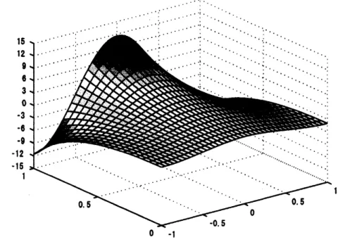
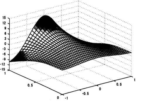
The solutions $u_{\Phi_{2}}$ obtainedby using different

noisy data with noise level $\delta=0,1,5,10$ are given in Figure 2-Figure 5,

respectively.

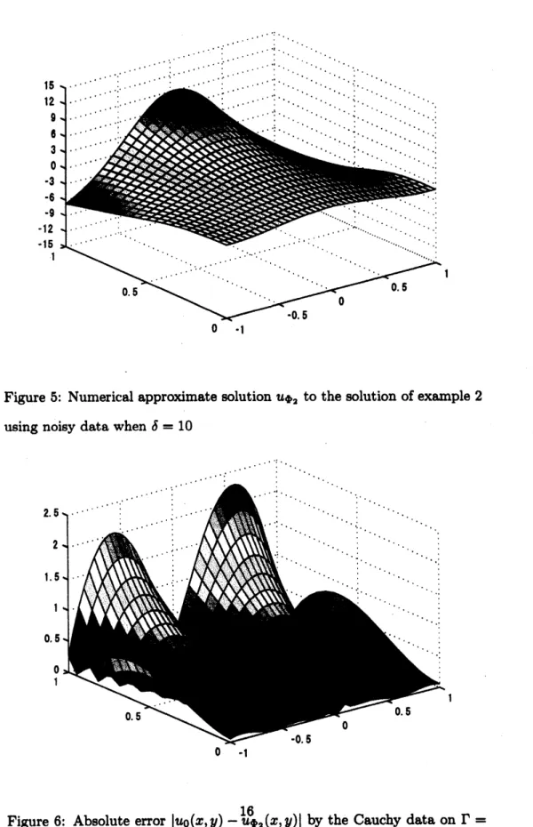
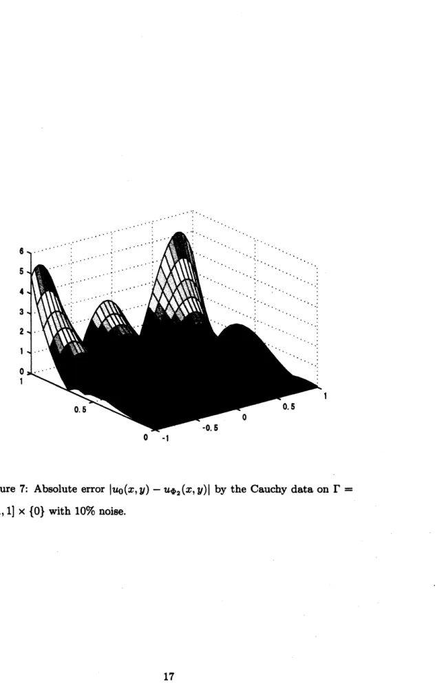
In order tostudy the errorprofiles ofour numerical solution to $u_{\Phi_{2}}$, in

Figure 6 and Figure 7, wedraw the absoluteerror

$E_{a}(x,y)$ $:=|u_{0}(x, y)-u_{\Phi_{2}}(x, y)|$, $(x, y)\in\Omega$

.

In this experiment, the noise level is set to be $\delta=10$ and both Example 1

and Example 2

are

tested. We observe that the

errors

becomes larger

near

the boundary $\Sigma$ in the bothexamples. This corresponds to the conditional stability estimate up to the boundary as

we

stated in Theorem 6 where the rate of the convergence to the exact solution is only logarithmic. By

the interior conditional stability estimate for Cauchy problem [6],

we

may

(10)

small part of thesubset$w\subset\Omega$whose boundary$\partial w$doesnot touch $\Sigma$

.

In [8],

thereconstruction

was

done in

a

subdomain$\omega$ for the

same

Cauchyproblem

for the Laplaceequation. For comparisons,

we

choose the

same

subdomain

$w$:

$w$ $:= \{(x,y);y+0.6(\frac{x}{0.6})^{2}-0.6\leq 0, y\geq 0\}$

and consider the relative

error

in $w$

$e_{r}(ua_{i})$ $:= \frac{||u_{0}-u_{\Phi_{1}}||_{L^{2}(w)}}{||u_{0}||_{L^{2}(w)}}$

,

$i=1,2$

.

In Table 2,

we

can see

that all the accuracies have improved.

Finally,

we

compute the numerical approximate solution to$u_{0}$when the

Cauchy data is given

on

the boundary$\Sigma=\{(x, 1);x\in[-1,1]\}$

.

Table 3 and

Table 4 show the relativeerrors in eachdomain respectively.

Examplel Example2

$N_{0}i_{S}ee$ $E_{r}(u_{l_{1}})$ $E_{r}(u_{\Phi_{2}})$ $E_{r}(u_{\Phi_{1}})$ $E_{r}(u_{\Phi_{2}})$

0% 0.0428 0.0338 0.0919 0.0667

1% 0.0507 0.0606 0.1099 0.0781

5%

02449

02340

03055

03186

10% 0.2797 0.2682 0.3410 0.3149

Table

1:

The relative

errors

$u_{\Phi_{j}}i=1,2$

on

the whole domain $\Omega$ when the Cauchy data

are

given

on

the boundary $\Gamma=[-1,1]x\{0\}$

.

(11)

Examplel Example2 $N_{0}i_{S}eee_{r}(u_{\Phi_{1}})e_{r}(u_{\Phi_{2}})e_{r}(u_{\Phi_{1}})e_{r}(u_{\Phi_{2}})\ovalbox{\tt\small REJECT}$ 0%

0.0044

0.0040

0.0023

0.0019

1% 0.0041 0.0074 0.0072 0.$W52$ 5% 0.0717

0.0677

0.0638 0.0786 10%

00879

00830 00768 00763

Table 2: The relative

errors

$u_{\Phi_{j}},$ $i=1,2$, in the interior part $w$ where the

Cauchydata is given onthe boundary $\Gamma=[-1,1]x\{0\}$

.

Examplel Example2 $N_{0}i_{See}$ 0% $0.\mathfrak{X}69$ $0.m43$ 0.0037 $0.\mathfrak{w}u$ 1% 0.0153 0.0106 0.0166 0.0046 5% 0.0375 0.0218 0.0361 0.0198 10% 00414 00425 00539 00292

errors

$u_{\Phi_{:}},$ $i=1,2$, onthe whole domain $\Omega$ wherethe

Cauchydata is given

on

the boundary $\Gamma$ such that _{$\partial\Omega\backslash \Gamma=[-1,1]x\{1\}$}

.

References

[1] N. Aronszajn, Theory of reproducingkernels, Rans. Amer. Math. Soc.

68 (1950) _337-404.

[2] J. Cheng, Y. C. Hon, T. Wei, M. Yamamoto, Numerical computation

ofa Cauchy problem for Laplace’s equation, ZAMM Z. Angew. Math. Mech. 81 (10) (2001) $66\triangleright 674$

.

[3] H. W. Engl, M. Hanke, A. Neubauer, Regularization of inverse

prob-lems, vol. 375 ofMathematics and its Applications, Kluwer Academic

Publishers Group, Dordrecht, 1996.

[4] C. W. Groetsch, The theory of Tikhonov regularization for Fredholm

equationsofthe first kind, vol. 105 of Research Notes inMathematics,

(12)

Examplel Example2

$N_{0}i_{S}ee$ $e_{r}(u_{\Phi_{1}})$ $e_{r}(u_{\Phi_{2}})$ $e_{r}(u_{\Phi_{1}})$ $e_{r}(u_{\Phi_{2}})$

0% $0$

0012

$0$0010 0.0034 0.0037

1% 0.0078

0.0054

0.0078

0.0046

5% 0.0176 0.0098

0.0276

0.0115

10% 0.0207 0.0200

0.0406

0.0138

errors

$u_{\Phi_{i}},$ $i=1,2$

,

in the interior part $w$ where the

Cauchydata is given onthe boundary$\Gamma$ such that _{$\partial\Omega\backslash \Gamma=[-1,1]x\{1\}$}

.

[5] D. N. H\‘ao, D. Lesnic, The Cauchy problemfor Laplace’s equationvia the conjugate gradient method, IMA J.Appl. Math. 65 (2) (2000)

199-217.

[6] V. Isakov, Inverse problems for partial differential $equation8$, vol. 127

of Applied Mathematical Sciences, 2nd ed., Springer, NewYork, 2006.

[7] E. J. Kansa, Multiquadrics–a scattered data approximation scheme with applications to computational fluid-dynamics. II. Solutions to parabolic, hyperbolic and eniptic partial differential equations,

Com-put. Math. Appl.

19

(8-9) (1990) 147-161.

[8] M. V. Klibanov, F. Santosa, A computational quasi-reversibility

method for Cauchy problems for Laplace’s equation, SIAM J. Appl.

Math. 51 (6) (1991) 1653-1675.

[9] R. Lattbs, J.-L. Lions, The method of quasi-reversibility. Applications

to partial differential equations, vol. 18 of Translated Bom the French

edition and edited by Richard Bellman. Modern Analytic and

Com-putational Methods in Science and Mathematics, American Elsevier

Publishing Co., Inc., NewYork, 1969.

[10] H.-J. Reinhardt, H. Han, D. N. H\‘ao, Stability and regularization ofa

discrete approximation to the Cauchy problem for Laplace’sequation,

SIAM J. Numer. Anal; ₃₆ _{(3) (1999)} $89b905$ (electronic).

[11] S. Saitoh, Theory ofreproducing kernels and its applications, vol. 189

of Pitman Research Notes in Mathematics Series, Longman Scientific

(13)

[12] T. Takeuchi, Y. Yamamoto, Tikhonov regularization by areproducing

kernel Hilbert space for the Cauchy problem for

an

elliptic equation,

UTMS Preprint Series 2007, UTMS 2007-2, University of Tokyo.

[13] A. N. Tikhonov, V. Y. Arsenin, Solutions of ill-posed problems, V. H. Winston

&Sons,

Washington, D.C.: John Wiley&Sons, New York,

1977, translated from the Russian, Preface by translation editor Fritz

John, Scripta Series in Mathematics.

[14] H. Wendland, ScatteredData Approximation, Cambridge Monographs

on

Applied and Computational Mathematics (No. 17),Cambridge

(14)

Figure 1: Surface plot for the function$u_{0}(x,y)=\cos\pi x$cosh$\pi y$ in example

2.

(15)

Figure3: Numericalapproximate solution $u_{\Phi_{2}}$ to the solution of example 2

using noisy data when $\delta=1$

(16)

Figure 5; _{Numerical approximate solution}$uo_{2}$ to the solution ofexample 2

using noisydata when $\delta=10$

16

(17)

Figure 7: Absolute error

₁

$u_{0}(x, y)-u_{\Phi_{2}}(x, y)|$ by the Cauchy data on $\Gamma=$