Analysis of Dynamics in Two-prey, one-predator
model: Effect of the Remained
carcass
岡山大学環境学研究科
李聖林
(Sungrim
Seirin
Lee)
Graduate School of Environmental Science,
Okayama
University
1
Introduction
The purpose of this paper is to propose the model which describes the effect of
remained
carcasses
and study the persistence and the dynamics. We suppose that the remainedcarcass
of a prey becomes foods of outsider species after predatorshave consumed the prey. It is well-known that many carnivorous insects such
as
ericket eat not only vegetable but also the
carcass
of small animals.For convenience, henceforth the prey will be called the existent prey and the
outsider species such as carnivorous insects, the existent prey. The variables of
$h_{1}(t),$ $h_{2}(t)$ and $p(t)$ denote the densities of the existent prey, the invader prey and
the predator respectively. In this paper, we consider
as
the following functionalresponse of the existent prey to the benefit of.remained
carcasses:
$\Psi(h_{1}, h_{2},p)=\frac{\tau_{1}h_{2}p}{\tau_{2}h_{1}+\tau_{\delta}h_{2}}$,
where $\tau_{1},$$\tau_{2}$ and $\tau_{3}$ are positive constants. we suppose that existent preys have two
negative effects by the intra-specics competition of themselves and the obstruction of invader preys, to have remained $ca\iota\cdot casses$. We $assu_{\wedge}^{-}\iota 1e$ that the two negative
effects are proportional to the density of the existent prey and the density of the invaderpreyrespectively, andfor simplifying the model, thereal amount ofremained
carcasscs which the existentpreyhas is proportional to thetotalamoimtofrpmained
carcasses
divided by the negative effects.Hence, Incorporating the functional response $\Psi$ in the existent prey, the model
takesthe form:
$\frac{d}{dt}\prime_{1_{1}},=\epsilon_{1}(1-\frac{h_{i}}{k_{1}})f_{t_{1}},-a_{1}h_{1}p+\frac{\tau_{1}h_{2}p}{\tau_{2}h_{1}+\tau_{3}h_{2}}h_{1}$
$\frac{d}{dt}h_{2}=\epsilon_{2}(1-\frac{h_{2}}{k,2})h_{2}-a_{2}h_{2}p$ (1)
wherc
$\epsilon_{i}$ growth rate of preys in the absence of predator
$k_{i}$ carrying capacity of
preys
$a_{i}$ consumption rate of
preys
by predator$b_{i}$ rate ofincrease in the number of predators from ingesting prey
$\delta$
death
rate ofpredator,and$\epsilon_{i},$ $k_{i},$$a_{i},$$b_{i}$ and $\delta$
are
positive constants. Now to avoid mathematicalcomplexity,we
nondimensionlize
the system(l) without loss ofgenerality :$\frac{d}{dt}y_{1}=(1-y_{1})y_{1}-\alpha_{1}y_{1}p+\frac{\omega y_{2}p}{ky_{1}+y_{2}}y_{1}$
$\frac{d}{dt}y_{2}=\epsilon(1-y_{2})_{l_{2}}/-\alpha_{2}y_{2}p$ (2) $\frac{d}{dt}p=-\gamma p+\beta_{1}y_{1}p+\beta_{2}y_{2}p$
where
$\alpha_{i}=\frac{a_{i}}{\epsilon_{1}}$, $\omega=\frac{\tau_{1}}{\epsilon_{1}}$, $k=\tau_{2^{\frac{k_{1}}{k_{2}’}}}$ $\epsilon=\frac{\epsilon_{2}}{\epsilon_{1}}$,
$\gamma=\frac{\delta}{\epsilon_{1}}$ and $\beta_{i}=\frac{b_{i}k_{i}}{\epsilon_{1}}$. (3)
In this paper,
we
suppose that(I) The existent preyand the predator have already approached tostable
coexistence density before the invader prey invade.
(II) The gain of the existent prey given by the predator is less than loss
when the existent prey and the invader prey approach their carrying
$capacitics$ rcspectively.
These assumptions lead to the following mathematical assumptions and initial
con-dition:
$1> \frac{\gamma}{\beta_{1}}$, (4)
$\frac{\omega}{k+1}<\alpha_{J}$ (5)
and
$(y_{1}(0), y_{2}(0),p(0))=( \frac{\gamma}{\beta_{1}},$ $n_{0},$$\frac{1}{\alpha_{1}}(1-\frac{\gamma}{\beta_{1}}))$ . (6)
2
Analysis
and Dynamics of
the
model
2.1
’Steady
states
and
Linear stability
In this section,
we
analyse stability of equilibria of system(2). On the boundary of$(1, 0,0),$ $E_{2}=(0,1,0),$$E_{3}=(1,1,0)$
$E_{4}=.( \overline{y}_{J}, 0,\overline{p})=(\frac{\gamma}{\beta_{1}})0,$ $\frac{1}{\alpha_{1}}(1-\frac{\gamma}{\beta_{1}}))$
since $\beta_{1}>\gamma$ from condition(4). The equilibrium
$E_{5}=(0,\overline{y}_{2},\tilde{p})=(0,$$\frac{\gamma}{\beta_{2}},$ $\frac{\epsilon}{\alpha_{2}}(1-\frac{\gamma}{\beta_{2}}))$
exists if $\beta_{2}>\gamma$. We $suImllarize$ the results of linear stability analysis
for these
equilibria.
1.$E_{0},$ $E_{1},$ $E_{2}$ and $E_{3}$ are saddle points and
so ar
$eun_{L}stable$. (7)2. $E_{4}$ is locally asymtotically stable if $\epsilon-\frac{\alpha_{2}}{\alpha_{1}}(1-\frac{\gamma}{\beta_{1}})<0$,
but is unstable if $\epsilon-\frac{\alpha_{2}}{\alpha_{1}}(1-\frac{\gamma}{\beta_{1}})>0$
.
(8)3. $E_{5}$ is locally asymtotically stable if $1+ \frac{\epsilon}{\alpha_{l}\prime}(\omega-\alpha_{1})(1-\frac{\gamma}{\beta_{2}})<0$,
but is unstable if $1+ \frac{\epsilon}{\alpha_{2}}(\omega-\alpha_{1})(1-\frac{\gamma}{\beta_{2}})>0$
.
(9)We note here that the equilibrium $E_{4}=(\overline{y}_{1},0,\overline{p})$ is initial condition in
our
Inodel.Thus if it is unstable, invader preys can succeed in invading even if $t$}$\iota e$ density of
the invader prey is very small.
We write the equilibrium of which all the coordinates
are
positive as $E^{*}=$$(y_{1}^{*}, y_{2}^{*}, p^{*})$, and then say that $\Gamma\prec_{\text{ノ^{}*}}$ is an interior
equilibrium. Now, we state the
existence and uniqueness of the interior equilibrium $E^{*}$ of system (2) $1^{\cdot}nder$ the conditions that the equilibria $E_{4}$ and $E_{5}$ are unstable.
Proposition 1 There exists the interior equilibrium $E^{*}=(y_{1}^{*}, y_{2}^{*},p^{*})$ of system
(2) uniquely if and only if the condition (8) and (9) are satisfied.
We
obtainthe
existenceof
the equilibrum point $E$“, but applications ofRouth-Hurwitz criterion give rise to complex set of mathematical conditions for stability
drawn
$hom$ these. In fact, when the linearization matrixon
$E^{*}$ leads to the eigen-value equation $\lambda^{3}+A_{1}\lambda^{2}+A_{2}\lambda+A_{3}=0$, Routh-Hurwitz criterion gives that all ofeigenvalues have negative real part if and only if
$A_{1}>0$, $A_{3}>0$ and $D=A_{1}A_{2}-A_{3}>0$.
We have $A_{1}>0$ and $A_{3}>0$ but the sign of $D$ depends onparameters. Bynumerical
simulations, wo find out Hope bifurcation for
some
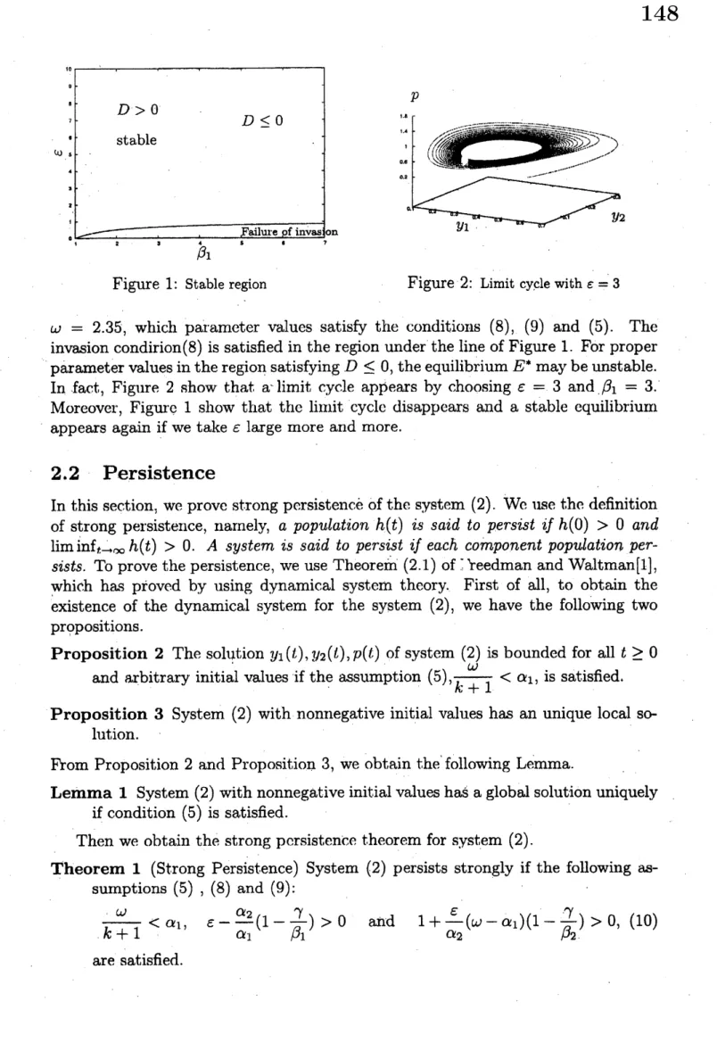
parameter values. For instancc,Figure 1 show that the stable region of the interior equilibrium $E^{*}$ for parameters
$\epsilon$ and $\beta_{1}$. We carry out numerical simulation for parameters $\epsilon$ and $\beta_{1}$ with the
$p$
Figure 1: Stable region Figure 2: Limit cyclewith $\epsilon=3$
$\omega=2.35$, which parameter values satisfy the conditions (8), (9) and (5). The
invasion condirion(8) is satisfied in the region under the line of Figure 1. For proper
parameter valuesinthe region satisfying$D\leq 0$, the equilibrium$E^{*}$ may be unstable.
In fact, Figure 2 show that $a$.limit $cycJ.e$ appears by choosing $\epsilon=3$ and $\beta_{1}=3$
.
Moreover, Figure 1 show that the $1i_{lI1}it$ cycle disappears and a stable equilibrium
appears again if we take $\epsilon$ large more and more.
2.2
Persistence
In this section,
we
prove strong pcrsistencc of the system (2). We $\iota xse$ the definitionof strong persistence, namely,
a
population $h(t)$ is said to persistif
$h(O)>0$ and$\lim\inf_{f,arrow\infty}h(t)>0.$ A system is said to persist
if
each component populationper-sists. To prove the persistence, we
use
Theorem (2.1) of$\vee\urcorner:reedman$ and Waltman[l],which has proved by using dynamical system theory. First of all, to obtain the existence of the dynamical system for the system (2),
we
have the following twopropositions.
Proposition 2 The
solution
$y_{1}(t),$$y_{2}(l),p(t)$ of system (2) is bounded for all $t\geq 0$and arbitrary initial values if the assumption (5),$\frac{\omega}{k+1}<\alpha_{1}$, is satisfied.
Proposition 3 System (2) with nonnegative initial values has
an
unique localso-lution.
Rom Proposition 2 and Proposition 3, we obtain the following Lemma.
Lemma 1 System (2) w\’ithnonnegative initialvalues has a global solutionuniquely
if condition (5) is satisfied.
Then
we
obtain the strong persistence theorem for system (2).Theorem 1 (Strong Persistence) System (2) persists strongly if the following
as-sumptions (5) , (8) and (9):
$\frac{\omega}{k+1}<\alpha_{1}$, $\epsilon-\frac{\alpha_{2}}{\alpha_{1}}(1-\frac{\gamma}{\beta_{1}})>0$ and $1+ \frac{\epsilon}{\alpha_{2}}(\omega-\alpha_{1})(1-\frac{\gamma}{\beta_{2}}.)>0,$ (10)
2.3
Numerical simulation results I
In this section, we study the dynamics of system (2)
more
detail by using numerical simulations. We assume
the conditions (4), (5) and $\beta_{2}>\gamma$, then the conditions (8)and (9) are rewritten for the parameter $\epsilon_{c}\backslash s$ the following:
$\frac{\alpha_{2}}{\alpha_{J}}(1-\frac{\gamma}{\beta_{1}})<\epsilon<\frac{\alpha_{2}}{(\alpha_{1}-\omega)(1_{\beta_{2}}-\lambda)}$ for $\alpha_{1}>\omega$, (11) $\epsilon>\frac{\alpha_{2}}{\alpha_{1}}(1-\frac{\gamma}{\beta_{1}})$ for $\frac{\omega}{k+1}<\alpha_{1}\leq\omega$
.
(12)On these cases, the invader prey succeed in invading and the extinction point of
the existent prey, $E_{5}$, is unstable. Moreover, these conditions guarantee the strong persistence of three species.
We choose parameter values satisfying persistence condition (10), and carry out$\cdot$
numerical simulations. Then we find out that populations of the system (2) have
a
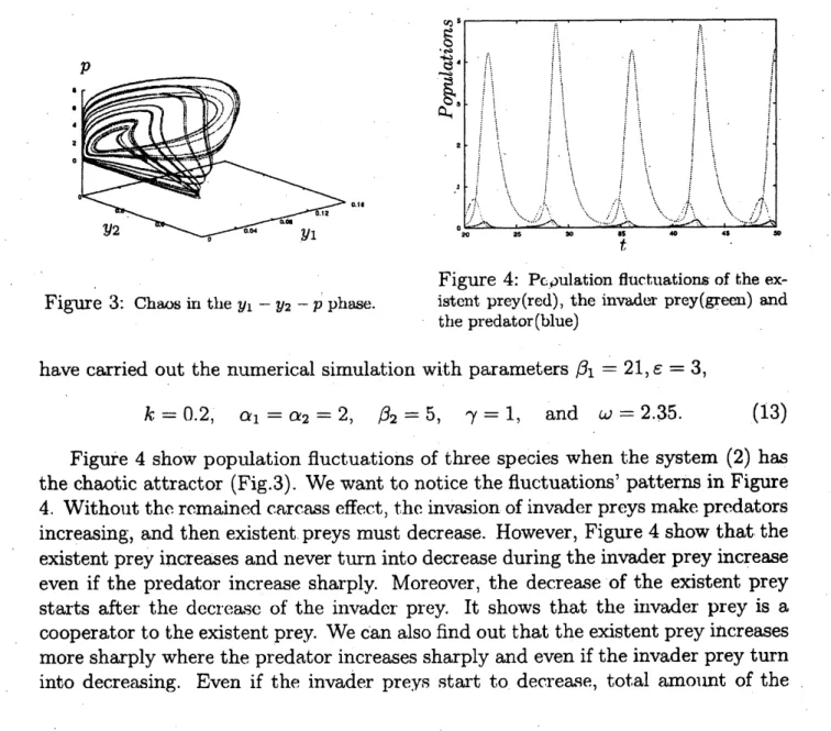
chaotic attractor. An example of thc chaotic attractor is shown in Figurc 3. WeFigure 4: $Pc_{I}$)$ulation$ fluctuations of the
ex-Figure 3: Chaosin the $y_{1}-y_{2}-p_{1)}h\prime asc^{\backslash }$. istcnt prey(rcd), the invader prcy(green) and
the predator(blue)
have carried out the numerical simulation with parameters $\beta_{1}=21,$$\epsilon=3$,
$k=0.2$, $\alpha_{1}=\alpha_{2}=2$, $\beta_{2}=5$, $\gamma=1$, and $\omega=2.35$. (13)
Figure 4 show population fluctuations of three species when the system (2) has
the chaotic
attractor
(Fig.3). Wewant to notice the fluctuations’ patterns in Figure4. Without the rcmaincdcarcass effect, the invasion of invaderpreys make predators increasing, and then existent preys must decrease. However, Figure 4 show that the
existent prey increases and
never
turn intodecrease during the invader prey increaseeven
if the predator increase sharply. Moreover, the decrease of the existent prey starts after the $dec1^{\cdot}e^{t}A^{\neg},C^{\backslash }$ of the invader prey. It shows that the invader prey isa
cooperator to the existent prey. We
can
also find out that the existent preyincreasesmore
sharply where the predatorincreases sharply andeven
if the invader prey turn into decreasing. Even if the invader preys start to decrease, total $\epsilon\prime lmotlnt$ of theremained $cal\cdot cass$ does not change very if the predators increase sufficiently. Thus
the existent prey can have enough amount of the remained carcasses to increase its
density. The predator and the existent prey have a symbiosis interaction.
3
Conclusions
In this paper, we have studied population dynamics of the two-prey, one-predator model which describes the effect of remained
carcasses.
The simple two-prey,one-predator Lotka-Volterra model has aglobally asymptotic stableinteriorequilibrium.
Thus, the dynamics ofthe model always gocs to stablc coexistcnt equilibrium $p^{\backslash }oint$.
However,
we
have shown that theremained carcass
$effe\neg.t$ gives very complexdy-namics under the strong persistent condition (10). Until now, many prey-predator
populationmodels have been studied but usually, they didnotconsider thecxistence ofthe remained carcass. It will be very important to consider the remained
carcass
effect in the interactions of species, especially in multi-species models.
References
[1] Fteedman H.I, Waltman P. Persistence in models of three interacting