On Convergence of the dqds and mdLVs Algorithms for Computing Matrix Singular Values(Mathematical Sciences for Large Scale Numerical Simulations)

On Convergence of the

dqds and

mdLVs

Algorithms

for

Computing

Matrix

Singular

Values

東京大学大学院 数理情報学専攻 相島 健助 (Kensuke Aishima)

松尾 宇泰 (Takayasu Matsuo)

室田 一雄 _(Kazuo Murota)

杉原 正顯 (Masaakl Sugihara)

Graduate School of Information Science and Technology, University of Tokyo

Abstract

Convergence $th\infty rems$ are established with mathematical rigour for two

algo-rithms forthe computationofsingular valuesofbidiogonal matrices: the differential

quotient difference with shift (dqds) and the modified discrete Lotka-Volterrawith shift (mdLVs). For the dqds algorithm, global convergence is guaranteed under a

fairly general assumption on the shift, and the asymptotic rate of convergence is

1.5 for the Johnson bound shift. Also for the mdLVs algorithm, globalconvergence is guaranteed in a realistic assumption, a substantial improvement of the

conver-gence analysis by Iwasaki and Nakamura. The asymptotic rate of convergenoe of

the mdLVs algorithm is 1.5 when the Johnson bound shift isemployed. Numerical

examples support these theoretical results.

1

Introduction

Every $n\cross m$ real matrix $A$ (with rank$(A)=r$)

can

be decomposed into

$A=U\Sigma V^{T}$

by suitable orthogonal matrices $U\in R^{nxn}$ and $V\in R^{mxm}$, where

$\Sigma=(\begin{array}{ll}D O_{r,m-r}O_{n-r,r} O_{n-r_{\prime}m-r}\end{array})$ _{$D=diag(\sigma_{1}, \ldots, \sigma_{r})$}

.

The values $\sigma_{1}\geq\cdots\geq\sigma_{r}>0$

are

the singular values of $A$

.

In the computation of matrix singular values, amatrix is often transformed first to

an

upper bidiagonal matrix by appropriate orthogonal matrices, and then its singular values

are calculated by some iterative algorithm. A common iterative algorithm for bidiagonal

matrices is the differential quotient difference with shift (dqds) algorithm [7]. The dqds is

now

implementedas DLASQinLAPACK [3, 10, 13] and widely usedbymanypractitioners

because of its high accuracy, speed, and numerical stability. The dqds is integrated into

Multiple Relatively Robust Representations $(MR^{3})$ algorithm [4, 5, 6]. On the otherhand,

shift (mdLVs) algorithm, was proposed [11], and has been rapidly expanding its influence

due to its high efficiency comparable to the dqds.

The aim of this report is to investigate the theoretical aspects of the two iterative

algorithms. So far, the convergence for the dqds has been proved only under the condition

that the shift is off. Independently of that, the rate of convergence has been shown to be

locally quadratic

or

cubic when the shift satisfies

some

stringent assumptions [7]. In this

report, we first prove that the dqds always converges as far as the shift satisfies acertain

natural condition. Then we show that, if the shiftis determined by the Johnson bound [9],

the asymptotIcrate ofconvergence is 1.5. For the mdLVs, aconvergence theoremis known

under a certain condition

on

the shift, and the local rate of convergence has been shown

to be quadratic

or

cubic under certain conditions. In this report

we

establish a stronger

convergence theorem for

a

wider class of shift choices, and also show that, with the shift

by the Johnson bound, the asymptotic rateof convergence is also 1.5.

2

Problem setting

We

as

sume

that the given real matrix $A$ has already been transformed to

a

bidiagonal

matrix

$B=(\begin{array}{llll}b_{1} b_{2} b_{3} \ddots \ddots b_{2m-2} b_{2m-1}\end{array})$ , (1)

to which the dqds or the mdLVs algorithm is applied.

Following [7], we

assume

Assumption (A) The bIdiagonal elements of $B$

are

positive, i.e., _{$b_{k}>0$} for

$k=1,2,$ $\ldots,$$2m-1$

.

This assumption guarantees (see [12]) that the singular values of $B$

are

all distinct: $\sigma_{1}>$

$...>\sigma_{m}>0$

.

Assumption (A) is not restrIctive, in theory

or

in practice. In fact, if a subdiagonal

element is zero, i.e., $b_{2k}=0$ for

some

$k$, then the problem reduces to two independent

problems

on

matrices of smaller sizes, $k\cross k$ and $(m-k)\cross(m-k)$

.

If there is

a

zero

element

on

the diagonal, several iteratIons of the dqd algorithm (I.e., the dqds algorithm

without shifts) suffioe to

remove

the diagonal zero, and the problem is again separated

into a set of smaller problems (see [7] for details). Finally it is easy to

see

that the singular

values

are

invariant if$b_{k}$ is replaced by

1

$b_{k}|$

.

In

our

problem setting

we

have assumed real matrices, whereas the singular value

decomposition is also defined for complex matrices. Our restrlction to real matrices is

justified by the fact that any complex matrix

can

be transformed to a real bidiagonal

matrix by, say, (complex) Householder transformations, while keeping its singular values

3Convergence

of

the

dqds Algorithm

In thissection, convergence results for the dqds algorithm are established with

mathemat-ical rigour. See [1] for the proofs.

3.1

The dqds algorithm

The dqds algorithm

can

be described in computer program form

as

follows.

Algorithm 3.1 The dqds algorithm

$\overline{Initialization:q_{k}^{(0)}=(b_{2k-1})^{2}(k=1,2,\ldots,m);e_{k}^{(0)}=(b_{2k})^{2}(k=1,2,\ldots,m-1)}$

1: for $n$ $:=0,1,$$\cdots$ do

2: choose shift $s^{(n)}(\geq 0)$

3: $d_{1}^{(n+1)}$ $:=q_{1}^{(n)}-s^{(n)}$ 4; for _$k:=1,$ $\cdots$ ,$m-1$ do $56:7$ $q^{(n+1)}p_{n+1)}:=d_{k}^{(n+1)}+e_{f}^{(n)}d_{k+1}:=d_{k}q_{k+1}/q_{k}-s^{(\mathfrak{n})}e_{k}:=e_{k}^{(n)}q_{k+1}^{(n)}/q_{k}n+1$) 8: end for 9: $q_{m}^{(n+1)}:=d_{m}^{(n+1)}$ 10: end for

The outermost loop is terminated when

some

suitable convergence criterion, say,

il

$e_{m-1}^{(n)}||\leq\epsilon$ for some prescribed constant $\epsilon>0$, is satisfied. At the termination we

have

$\sigma_{m}^{2}\approx q_{m}^{(n)}+\sum_{l=0}^{n-1}s^{(l)}$ (2)

and hence $\sigma_{m}$

can

be approximated by

$\sqrt{q_{m}^{(n)}+\sum_{l--0}^{n-1}s^{(l)}}$

.

Then by the deflation process

theproblem is shrunk to an $(m-1)\cross(m-1)$ problem, and the

same

procedure isrepeated

until $\sigma_{m-1},$ _$\ldots,$$\sigma_{1}$ are obtained inturn.

It turns out to be convenient to introduce additional notations $e_{0}^{(n)}$ and $e_{m}^{(n)}$ with

“boundary conditions”:

$e_{0}^{(n)}=0$, $e_{m}^{(n)}=0$ $(n=0,1, . )$

to simplify the expression of the algorithm. Put

$b_{k}^{(0)}=b_{k}(k=1,2, \ldots, 2m-1)$_{, and}

$q_{k}^{(n)}$ _$=$ $(b_{2k-1}^{(n)})^{2}$ $(k=1,2, \ldots, m;n=0,1, \ldots)$, (4)

$e_{k}^{(n)}$ _$=$ $(b_{2k}^{(n)})^{2}$ $(k=1,2, \ldots, m-1;n=0,1, \ldots)$

.

(5)

Then Algorithm3.1 canbe rewritten interms of the Cholesky decomposition (with shifts):

$(B^{(n+1)})^{T}B^{(n+1)}=B^{(n)}(B^{(n)})^{T}-s^{(n)}I$, (6)

where $B^{(0)}=B$

.

_{Rom (6) it follows that}

$(B^{(n)})^{T}B^{(n)}=W^{(n)}((B^{(0)})^{T}B^{(0)}- \sum_{l=0}^{n-1}s^{(l)}I$

ノ

$(W^{(n)})^{-1}$, (7)

where $W^{(n)}=(B^{(n-1)}\cdots B^{(0)})^{-T}$ is

a

nonsingular matrix. Therefore the eigenvalues of

$(B^{(n)})^{T}B^{(n)}$

are

the

same as

those of $(B^{(0)})^{T}B^{(0)}- \sum_{l=0}^{n-1}s^{(l)}I$

.

If $s^{(n)}<(\sigma_{\min}^{(n)})^{2}$ in each iteration

$n$, where $\sigma_{\min}^{(n)}$ is the smallest singular value of $B^{(n)}$,

the variables in the dqds algorithm

are

always positive so that the algorithm does not

break down as follows.

Lemma 3.1 (Positivityof the variablesin the dqds algorithm). Suppose the dqds algorithm

is applied to the $mat\dot{m}B$ satisfying Assumption (A).

If

$s^{(n)}<(\sigma_{\min}^{(n)})^{2}(n=0,1,2, \ldots)$,

then $(B^{(n)})^{T}B^{(n)}$

are

positive definite, and hence $q_{k}^{(n)}>0(k=1, \ldots , m),$ $e_{k}^{(\mathfrak{n})}>0(k=$

$1,$

$\ldots,$$m-1$), and$d_{k}^{(n)}>0(k=1, \ldots, m)$

for

$n=0,1,2,$$\ldots$.

$\blacksquare$

3.2

Global

convergence

of the dqds

algorithm

The next theorem establishes the convergence of the dqds algorithm. Moreover, the

theo-rem states that the variables $q_{k}^{(n)}$ converge to the square of the singular values minus the

sum

ofthe shifts, and that they are placed in the descending order.

Theorem 3.1 (Convergence of the dqds algorithm). Selppose the matric $B$

satisfies

As-sumption (A), and the

_shift

in the dqds algori thm is taken so that$0\leq s^{(n)}<(\sigma_{\min}^{(n)})^{2}$ holds

for

all$n$. Then

$\sum_{n=0}^{\infty}s^{(n)}\leq\sigma_{m}^{2}$

.

(8)

Moreover,

$\lim_{narrow\infty}e_{k}^{(n)}$ $=$ $0$ $(k=1,2, \ldots , m-1)$, (9)

$\lim_{narrow\infty}q_{k}^{(n)}$ $=$ $\sigma_{k^{2}}-\sum_{n=0}^{\infty}s^{(n)}$ $(k=1,2, \ldots, m)$

.

(10)

The next theoremstates the asymptotic rateofconvergence of the dqds algorithm. Let

us define

$\rho_{k}$ $=$ $\frac{\sigma_{k+1^{2}}-\sum_{n--0^{S}}^{\infty(n)}}{\sigma_{k^{2}}-\sum_{n=0}^{\infty}s^{(n)}}$ $(k=1, \ldots, m-1)$, (11)

.

$r_{k}^{(n)}$ _{$=$ $(q_{k}^{(n)}+ \sum_{l=0}^{n-1}s^{(l)})-\sigma_{k^{2}}$} $(k=1, \ldots, m)$. (12)

In view of (2), $r_{k}^{(n)}$ is the

error

in the approximated eigenvalue of _$B^{T}B$

.

Note that $0<$

$\rho_{k}<1$ $(k=1, \ldots , m-2)$, and _{$0<\rho_{m-1}<1$} if $\sigma_{m}^{2}-\sum_{n=0}^{\infty}s^{(n)}>0$ and _{$\rho_{m-1}=0$} if

$\sigma_{m}^{2}-\sum_{n=0}^{\infty}s^{(n)}=0$

.

Theorem 3.2 (Rate of convergence of the dqds algorithm). Under the same assumption

as

in Theooem 3.1,

we

have $n arrow\infty narrow\infty\lim_{\lim\frac{\frac{e_{k}^{(n+1)}}{r_{1}^{(n+1)}e_{k}^{(n)}}}{(n)}}$ $==\rho_{1}\rho_{k}$ $(k=1, \ldots, m-1)$, $(14)(13)$ $r_{1}$ $\lim_{narrow\infty}\frac{r_{m}^{(n+1)}}{r_{m}^{(n)}}$ $=\rho_{m-1}$

.

(15)

hrthermore,

_if

$\rho_{k-1}\neq\rho_{k}(k=2, \ldots, m-1)$, then

$\lim_{narrow\infty}\frac{r_{k}^{(n+1)}}{r_{k}^{(\mathfrak{n})}}=\max\{p_{k-1}, \rho_{k}\}$ $(k=2, \ldots, m-1)$

.

(16)

Therefore, $e_{k}^{(n)}$ $(k=1, \ldots , m-2)$ and $r_{k}^{(n)}(k=1, \ldots, m-1)$

are

of

linear convergence

as $narrow\infty$

.

The bottommost elements $e_{m-1}^{(n)}$ and $r_{m}^{(n)}$ are also

of

linear convergence when

$\rho_{m-1}>0,$ $i.e.,$ $\sigma_{m}^{2}-\sum_{n=0}^{\infty}s^{(n)}>0$, and

of

superlinear

conve

rgence when _{$\rho_{m-1}=0,$ $i.e.$},

$\sigma_{m}^{2}-\sum_{n=0}^{\infty}s^{(n)}=0$

.

Remark 3.1. When $\rho_{k-1}=\rho_{k}$, we have aweaker claim that

$r_{k}^{(n)}$ _$=$ $\frac{\sum_{l=n+1}^{\infty}e_{k-1}^{(l)}}{e_{k-1}^{(n+1)}}$

.

$e_{k-1}^{(n+1)}- \frac{\sum_{l=n}^{\infty}e_{k}^{(l)}}{e_{k}^{(n)}}$

.

$e_{k}^{(n)}$,

which implies that, for any small $\epsilon>0$,

$|r_{k}^{(n)}|\leq O((p_{k}+\epsilon)^{n})$ _{$(k=2, \ldots, m-1)$}

.

3.3

Convergence rate

of

the

dqds with the

Johnson

bound

(17)

In this section, we show that the asymptotic rate of convergence of the dqds algorithm

is 1.5 if the shift is determined by the Johnson bound [9]. Though the Johnson bound is

valid for a general matrix, we present here its version for a bidiagonal matrix $B$

.

Lemma 3.2 (Johnson bound [9]). For a matrix $B$

of

the

form

(1),

define

$\lambda=\min_{k=1,\ldots,m}\{|b_{2k-1}|-\frac{|b_{2k-2}|+|b_{2k}|}{2}I$ ,

where $b_{0}=b_{2m}=0$ and let $\sigma_{m}$ denote the smallest singular value

of

B. Then $\sigma_{m}\geq\lambda$

.

Moreover,

_if

the subdiagonal elements $(b_{2}, b_{4}, \ldots , b_{2m-2})$

are

nonzero, then $\sigma_{m}>\lambda$

.

$\blacksquare$

Withreference to (3), (4) and (5) we define the shift by the Johnson bound as follows:

$\lambda^{(n)}$

$=$ $\min_{k=1,\ldots,m}\{\sqrt{q_{k}^{(n)}}-\frac{1}{2}(\sqrt{e_{k-1}^{(n)}}+\sqrt{e_{k}^{(n)}})\}$ ,

$s^{(n)}$ _$=$ $( \max\{\lambda^{(n)}, 0\})^{2}$ . (18)

This choice of the shift guarantees the condition $0\leq s^{(n)}<(\sigma_{\min}^{(n)})^{2}$ in each iteration _$n$,

and hence the dqds is convergent by Theorem 3.1. The precise rate ofconvergence

can

be

revealed through a scrutiny of the shift.

The following theorem shows that therate ofconvergence ofthe dqds is 1.5. The

theo-rem

refers only to the lower right two elements of$B^{(n)}$, and the

error

in theapproximation

of the smallest eigenvalue of$B^{T}B$

.

This is sufficient from the practical point of view since

whenever the lower right elements converge to zero, the deflation is applied to reduce the

matrix size.

Theorem 3.3 (Rate of convergence of the dqds). Suppose the dqds algonthm with the

Johnson bound is applied to a matm $B$ that

satisfies

Assumption (A). Then we have

$\lim_{narrow\infty}\frac{e_{m-1}^{(n+1)}}{(e_{m-1}^{(n)})^{3/2}}=\frac{1}{\sqrt{\sigma_{m-1^{2}}-\sigma_{m}^{2}}}$, (19)

$\lim_{narrow\infty}\frac{q_{m}^{(n+1)}}{(q_{m}^{(n)})^{3/2}}=\frac{1}{\sqrt{\sigma_{m-1^{2}}-\sigma_{m^{2}}}}$, (20)

$\lim_{narrow\infty}\frac{r_{m}^{(n+1)}}{(r_{m}^{(n)})^{3/2}}=\frac{1}{\sqrt{\sigma_{m-1^{2}}-\sigma_{m^{2}}}}$

.

(21)

That is, the $mte$

of

convergence

is 1.5. $\blacksquare$

4

Convergence

of

the mdLVs

Algorithm

In this section,

convergence

results for the mdLVs algorithm

are

established with

4.1

The mdLVs algorithm

The mdLVs algorithm $[8, 11]$ can be described as follows.

Algorithm 4.1 mdLVs algorithm

$\overline{Initialization:w_{0}^{(0)}=0;w_{2m}^{(0)}=0;w_{k}^{(0)}=(b_{k})^{2}(k=1,2,\ldots,2m-1)}$

1: for $n:=0,1,$$\cdots$ do

2: choose shift $s^{(n)}(\geq 0)$ and parameter $\delta^{(n)}(>0)$ based on $w_{k}^{(n)}$

3: $u_{0}^{(n)}$ $:=0$; $u_{2m}^{(n)}$ $:=0$ 4: for_$(n)k:=1,$ $\cdots 2m-1$ do 5: $u_{k}$ $:=w_{k}^{(n)}/(1+\delta^{(n)}u_{k-1}^{(n)})$ 6;

end

for 7: $v_{0}^{(n)}$ $:=0$; $v_{2m}^{(n)}$ $:=0$ 8: for $k:=1,$$\cdots$ ,$2m-1$ do 9: $v_{k}^{(n)}$ $:=u_{k}^{(n)}(1+\delta^{(n)}u_{k+1}^{(n)})$ 10: end for 11: $w_{0}^{(n+1)}$ _$:=0$; $w_{2m}^{(n+1)}$ _$:=0$ 12: if $s^{(n)}>0$ then 13: for $k:=1,$ $\cdots m-1$ do 14: $w_{2k-1}^{(n+1)}$ $:=v_{2k-1}^{(n)}+v_{2k-2}^{(n)}-w_{2k-2}^{(n+1)}-s^{(n)}$ 15: $w_{2k}^{(n+1)}$ $:=v_{2k-1}^{(n)}v_{2k}^{(n)}/w_{2k-1}^{(n+1)}$ 16: end for 17: $w_{2m-1}^{(n+1)}$ $:=v_{2m-1}^{(n)}+v_{2m-2}^{(n)}-w_{2m-2}^{(n+1)}-s^{(n)}$ 18: else 19: for $k:=1,$$\cdots 2m-1$ do 20: $w_{k}^{(n+1)}$ $:=v_{k}^{(n)}$ 21: end for 22: end if 23: end for

The outermost loop is terminated when some suitable convergence criterion, say,

$\Vert w_{2m-2}^{(n)}\Vert\leq\epsilon$ for

some

prescribed constant $\epsilon>0$, is satisfied. At the termination

we

have

$\sigma_{m}^{2}\approx w_{2m-1}^{(n)}+\sum_{l=0}^{n-1}s^{(l)}$ (22)

and hence $\sigma_{m}$

can

be approximatedby $\sqrt{w_{2m-1}^{(n)}+\sum_{l--0}^{n-1}s^{(l)}}$. Thenby thedeflation process

the problem is shrunktoan $(m-1)\cross(m-1)$ problem, and thesame_procedureis repeated

until $\sigma_{m-1},$ _$\ldots,$$\sigma_{1}$ are obtained in turn. In Algorithm 4.1,

$\delta^{(n)}>0$ is

a

free parameter.

It turns out to be convenient to introduce

$w_{0}^{(n)}=w_{2m}^{(n)}=0$, $u_{0}^{(n)}=u_{2m}^{(n)}=0$, $v_{0}^{(n)}=v_{2m}^{(n)}=0$ (23) for $n=0,1,2,$$\ldots$ as boundary conditions.

Similarly to the dqds, we use the notation (3) with $b_{k}^{(0)}=b_{k}(k=1,2, \ldots, 2m-1)$_,

and put

$w_{2k-1}^{(n)}$ _$=$ $(b_{2k-1}^{(n)})^{2}$ $(k=1,2, \ldots, m;n=0,1, \ldots)$,

$w_{2k}^{(n)}$ _$=$ $(b_{2k}^{(n)})^{2}$ $(k=1,2, \ldots, m-1;n=0,1, \ldots)$

.

Again

we

denote by $\sigma_{\min}^{(n)}$ the smallest singular value of $B^{(n)}$

.

The next lemma states that

the algorithm does not break down if $s^{(n)}<(\sigma_{\min}^{(n)})^{2}$ in each iteration _$n$

.

Lemma 4.1 (PositIvity of the variables in the mdLVs algorithm). Suppose the $mdLVs$

algorithm is applied to the matrix $B$ satisfying Assumption (A).

If

$s^{(n)}<(\sigma_{\min}^{(n)})^{2}(n=$

$0,1,2,$ $\ldots$), then $(B^{(n)})^{T}B^{(n)}$

are

positive definite, and hence $u_{k}^{(n)}>0,$ $v_{k}^{(n)}>0$, and

$w_{k}^{(n)}>0(k=1, \ldots, 2m-1)$

_for

_$n=0,1,2,$

$\ldots$

.

$\blacksquare$

4.2

Global

convergence

of the mdLVs

A global convergence theorem for the mdLVs algorithm is available in [11]. The theorem,

however,

_assumes

_{not only} $0\leq s^{(n)}<(\sigma_{m}^{(n)})^{2}$ but also $\sum_{n=0}^{\infty}s^{(n)}<\sigma_{m}^{2}$ for the chosen

shift. It

can

easily besuspected from the convergence analysisfor the dqds algorithmthat

the latter assumption is not met whensuperlinear convergenceisrealized. As we

see

later,

this is in fact the

case

with the mdLVs algorithm with the Johnson bound shift. Thus

we

are motivated to establish a stronger convergence theorem that works also in the

case

of

$\sum_{n=0}^{\infty}s^{(n)}=\sigma_{m^{2}}$

.

The next theorem establishes the convergence of the mdLVs. Moreover, the theorem

states that the variables $w_{2k-1}^{(n)}$ converge to the square of the singular values minus the

sum of the shifts, andthat they

are

placed in the descending order.

Theorem 4.1 (Convergence of the mdLVs algorithm). Suppose the matrix $B$

satisfies

‘

Assumption (A), and the

_shift

in the $mdLVs$ algorithm is taken so that$0\leq s^{(\mathfrak{n})}<(\sigma_{\min}^{(n)})^{2}$

holds

_for

all $n$, and the pammeter is taken

so

that

$\lim_{n\Rightarrow\infty}\frac{1}{\delta^{(n)}}=D_{0}$ (24)

for

some

nonnegative constant $D_{0}\geq 0$

.

Then

we

have

$\sum_{n=0}^{\infty}s^{(n)}\leq\sigma_{m}^{2}$

.

(25)

Moreover,

$\lim_{narrow\infty}w_{2k}^{(n)}$ $=$ $0$ $(k=1,2, \ldots , m-1)$, (26)

$\lim_{narrow\infty}w_{2k-1}^{(n)}$ $= \sigma_{k^{2}}-\sum_{n=0}^{\infty}s^{(n)}$ $(k=1,2, \ldots, m)$

.

(27)

The next theorem states the asymptotic rate of convergence of the dqds algorithm.

Theorem 4.2 (Rateof convergence of themdLVs algorithm). Under the same assumption

as in Theorem 4.1, we have

$\lim_{narrow\infty}\frac{e_{k}^{(n+1)}}{e_{k}^{(n)}}=\frac{\sigma_{k+1^{2}}+D_{0}-\sum_{n--0}^{\infty}s^{(n)}}{\sigma_{k^{2}}+D_{0}-\sum_{n=0}^{\infty}s^{(n)}}<1$ $(k=1, \ldots, m-1)$

.

(28)

Therefore

$e_{k}^{(n)}$ $(k=1, \ldots , m-2)$

are

of

linear

convergence

as

_{$narrow\infty$}

.

The bottommost

el-ement$e_{m-1}^{(n)}$ is also

of

linear convergence when_{$\sigma_{m}^{2}+D_{0}-\sum_{n=0}^{\infty}s^{(n)}>0$}, and

of

superlinear

convergence when $\sigma_{m^{2}}+D_{0}-\sum_{n=0}^{\infty}s^{(n)}=0$

.

$\blacksquare$

4.3

Convergence

rate

of the mdLVs with the Johnson bound

(29)

For the mdLVs algorithm it is proposed in $[8, 11]$ to

use

the shift $s^{(n)}$ determined from the

Johnson bound as follows:

$\lambda^{(n)}$

$=$ $\min_{k=1,\ldots,m}\{\sqrt{w_{2k-1}^{(n)}}-\frac{1}{2}(\sqrt{w_{2k-2}^{(n)}}+\sqrt{w_{2k}^{(n)}})\}$ ,

$s^{(n)}$ _$=$ $( \max\{\lambda^{(n)}, 0\})^{2}$

.

(30)

The following theorem shows that the rate of convergence of the dqds is 1.5 if the

parameter $\delta^{(n)}$ satisfies

$\lim_{narrow\infty}\delta^{(n)}=+\infty$ (31)

as

well

as

another natural condition. Note that the condition (31) is aspecial

case

of (24)

with $D_{0}=0$

.

The theorem refers only to the lower right two elements of $B^{(n)}$

.

This is

sufficient from the practicalpoint ofview sincewhenever the lowerrightelementsconverge

to zero, the deflation is applied to reduce the matrix size.

Theorem

4.3

(Rate

of convergence

of the mdLVs). Suppose the mdLVs algorithm with

the Johnson bound is applied to

a

matrix$B$ that

satisfies

Assumption (A).

If

the parameter

$\delta^{(n)}$

satisfies

(31) and

$D_{1}\leq\delta^{(n)}w_{2m-2}^{(n)}$ _{$(n=1,2, \ldots)$} (32)

for

some

positive constant $D_{1}$,

we

have

$\lim_{narrow\infty}\frac{w_{2m-2}^{(n+1)}}{(w_{2m-2}^{(n)})^{3/2}}=\frac{1}{\sqrt{\sigma_{m-1^{2}}-\sigma_{m^{2}}}}$,

$\lim_{narrow\infty}\frac{w_{2m-1}^{(n+1)}}{(w_{2m-1}^{(n)})^{3/2}}=\frac{1}{\sqrt{\sigma_{m-1^{2}}-\sigma_{m}^{2}}}$

.

5

Numerical

experiments

In this section, simple numerical results

are

presentedto illustrate the theory. We consider

an

$m\cross m$ symmetric tridiagonal matrix

$T=(_{0}^{a}$ $b$ $ab$

.

$b$ $a0b$

),

(33)

the eigenvalues of which are

$a+2b \cos(\frac{\pi k}{m+1})$ $(k=1, \ldots, m)$

.

As

a test matrix, the bidiagonal matrix $B$ is obtained from the Cholesky decomposition

of$T$

.

The parameters

are

taken as _{$m=10,$ $a=1.0$} and _$b=0.2$

.

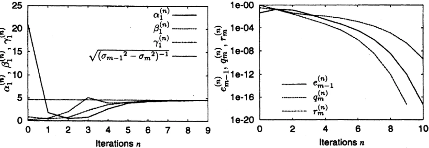
First

we

show the result with the dqds algorithm. In view of Theorem 3.3, we define

$\alpha_{1}^{(n)}=\frac{e_{m-1}^{(n+1)}}{(e_{m-1}^{(n)})^{3/2}}$, $\beta_{1}^{(n)}=\frac{q_{m}^{(n+1)}}{(q_{m}^{(n)})^{3/2}}$, $\gamma_{1}^{(n)}=\frac{r_{m}^{(n+1)}}{(r_{m}^{(n)})^{3/2}}$,

which should converge to the constant 1/$\sqrt{(\sigma_{m-1^{2}}-\sigma_{m^{2}})}$ according to the theory. The

result is shown in Figure 1. The solid line (–) shows $\alpha_{1}^{(\mathfrak{n})}$, the chained line (—–.)

shows $\beta_{1}^{(n)}$ and the

dashed-dotted line (-.-.-.) shows $\gamma_{1}^{(n)}$

.

The dotted line (–) shows

1/$\sqrt{(\sigma_{m-1^{2}}-\sigma_{m^{2}})}=4.60$

.

The solid line, the chained line and the dashed-dotted line all

approach the dotted line in Figure 1.

In Figure 2, $e_{m-1}^{(n)},$ $q_{m}^{(n)}$ and $r_{m}^{(n)}$

are

plotted in the single logarithmic graph. The

solid line shows $e_{m-1}^{(n)}$, the chained line shows $q_{m}^{(n)}$ the dashed-dotted line shows $r_{m}^{(n)}$. The

variables $e_{m-1}^{(n)},$ $q_{m}^{(n)}$ and $r_{m}^{(n)}$ converge

to

zero.

By FIgure 1 and Figure 2

we

can say that

the rate ofconvergence is 1.5.

Iterationsn lterations n

Figure 1: dqds algorithm: $\alpha^{(\mathfrak{n})},$ $\beta^{(n)}$ and$\gamma^{(n)}$

.

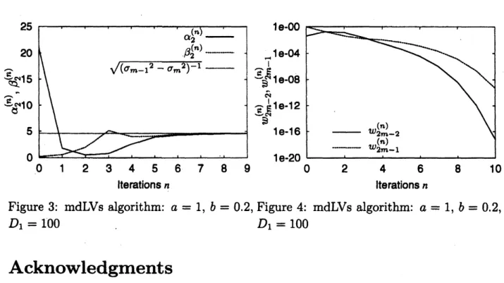
Figure2: dqds algorithm: $e_{m-1}^{(n)},$$q_{m}^{(n)}$ and$r_{m}^{(\mathfrak{n})}$

Second we show the result with the mdLVs algorithm. In view of Theorem 4.3, we

define

$\alpha_{2}^{(n)}=\frac{w_{2m-2}^{(n+1)}}{(w_{2m-2}^{(n)})^{3/2}}$, $\beta_{2}^{(n)}=\frac{w_{2m-1}^{(n+1)}}{(w_{2m-1}^{(n)})^{3/2}}$,

which should converge to the constant 1/$\sqrt{(\sigma_{m-1^{2}}-\sigma_{m^{2}})}$ according to the theory. We

chose the parameter $D_{1}=100$ in Theorem 4.3. The result is shown in Figure 3. The solid

line ($arrow shows\alpha_{2}^{(n)}$ and the chained line (——.) shows $\beta_{2}^{(n)}$

.

The dotted line $(arrow shows$

$1/\sqrt{(\sigma_{m-1^{2}}-\sigma_{m^{2}})}=4.60$

.

The solid line and the chained line approach the dotted line

in Figure 3.

In Figure 4, $w_{2m-2}^{(n)}$ and $w_{2m-1}^{(n)}$

are

plotted in the single logarithmic graph. The solid

line shows $w_{2m-2}^{(n)}$ and the chained line shows $w_{2m-1}^{(n)}$

.

The variables $w_{2m-2}^{(n)}$ and $w_{2m-1}^{(n)}$

converge to

zero.

By Figure 3 and Figure 4

we

can say that the rate ofconvergenoe is 1.5.

lterationsn lterationsn

Figure 3: mdLVs algorithm: $a=1,$ $b=0.2$, Figure 4: mdLVs algorithm: $a=1,$ $b=0.2$,

$D_{1}=100$ $D_{1}=100$

Acknowledgments

The authors are thankful to Yusaku Yamamoto for

a

number ofhelpful comments. Part

of this work is supported by the 21st Century COE Program

on

Information Science and

Technology Strategic Core and

a

Grant-in-Aid of the Ministry of Education, Culture,

Sports, Science and Technologyof Japan.

References

[1] K. Aishima, T. Matsuo, K. Murota and M. Sugihara: On Convergence of the dqds

Algorithm for Singular Value Computation, Mathematical Engineering Technical

Re-ports, METR 2006-59, University of Tokyo, November 2006.

[2] K. Aishima, T. Matsuo, K. Murota and M. Sugihara: On Convergence of dqds and

mdLVs Algorithms _for Singular Value Computation (in Japanese), submitted for

Pub-lication. (相島健助, 松尾宇泰, 室田一雄, 杉原正顯

:

特異値計算のための dqds 法

と mdLVs 法の収束性について, 投稿中.)

[3] E. Anderson, Z. Bai, C. Bischof, S. Blackford, J. Demmel, J. Dongarra, J. Du Croz,

A. Greenbaum, S. Hammarling, A. Mckenny and D. Sorensen: LAPA$CK$ Users’ Guide,

Third Edition, SIAM, 1999.

[4] I. S. Dhillon: A New $O(n^{2})$ Algorithm for the Symmetric Tridiagonal

Eigen-$value/Eigenvector$ Problem, Ph. D Thesis, Computer

Science

Division, University of

California, Berkeley, California,

1997.

[5] I. S. Dhillon and B. N. Parlett: Multiple Representations to Compute Orthogonal

Eigenvectors of Symmetric Tridiagonal Matrices, Linear Algebra and Its Applications,

vol. 387 (2004), pp. 1-28.

[6] I. S. Dhillon and B. N. Parlett: Orthogonal Eigenvectors and Relative Gaps, SIAM

Joumal on Matri Analysis and Applications, vol. 25 (2004), pp. 858-899.

[7] K. V. Fernando and B. N. Parlett: AccurateSingular Values and Differential qd

Algo-rithms, Numerische Mathematik, vol. 67 (1994), pp. 191-229.

[8] M. Iwasaki and Y. Nakamura: On Basic PropertIes of the dLV Algorithm for

Com-puting Singular Values (in JaPanese), $\pi_{ansactions}$

of

the

JaPan

Society

for

Industrial

and Applied Mathematics, vol. 15 (2005),

pp.

287-306. (岩崎雅史, 中村佳正 : 特異値

計算アルゴリズム dLV の基本性質について, 日本応用数理学会論文誌, vol. 15 (2005),

pp. 287-306.)

[9] C. R. Johnson: AGersgorin-type Lower Bound forthe Smallest SingularValue, Linear

Algebra and Its Applications, vol. 112 (1989), pp. 1-7.

[10] LAPACK, $http://www.netlib.org/lapack/$

[11] Y. Nakamura: Functional Mathematics

_for

IntegmbleSystems (In Japanese), Kyoritsu

Publishing Co., Tokyo,

2006.

(中村佳正:_{「可積分系の機能数理」,共立出版}, 2006.)

[12] B. N. Parlett: The Symmetric Eigenvalue Problem, Prentice-Hall, Englewood Cliffs,

New Jersey, 1980; SIAM, Philadelphia, 1998.

[13] B. N. Parlett and O. Marques: An Implementation of the dqds Algorithm (Positive