A SURVEY OF LENGTH SERIES IDENTITIES FOR SURFACES, 3-MANIFOLDS AND REPRESENTATION VARIETIES(Complex Analysis and Geometry of Hyperbolic Spaces)

A SURVEY OF LENGTH SERIES IDENTITIES FOR SURFACES,

3-MANIFOLDS AND REPRESENTATION VARIETIES

SER PEOW TAN, YAN LOI WONG&YING ZHANG

ABSTRACT. Wesurveysomeofourrecentresultsonlength seriesidentities for

hyperbolic (cone) surfaces, possibly with cusps $\mathrm{a}\mathrm{n}\mathrm{d}/\mathrm{o}\mathrm{r}$ boundary geodesics;

classical Schottky groups; $\mathrm{r}\mathrm{e}\mathrm{p}\mathrm{r}\mathrm{e}\mathrm{s}\mathrm{e}\mathrm{n}\mathrm{t}\mathrm{a}\mathrm{t}\mathrm{i}\mathrm{o}\mathrm{n}\mathrm{s}/\mathrm{c}\mathrm{h}\mathrm{a}\mathrm{r}\mathrm{a}\mathrm{c}\mathrm{t}\mathrm{e}\mathrm{r}\mathrm{s}$ of the one-holed torus

group to $\mathrm{S}\mathrm{L}(2, \mathrm{C})_{\mathrm{i}}$ and hyperbolic 3 manifolds obtained by hyperbolic Dehn

surgery on punctured torus bundles over the circle. These can be regarded

asgeneralizationsand variations of$\mathrm{M}\mathrm{c}\mathrm{S}\mathrm{h}\mathrm{a}\iota \mathrm{l}\mathrm{e}’ \mathrm{s}$identity for cusped hyperbolic surfaces, which has found some striking applications in the recent work of

Mirzakhani. Wediscugs _{some of the methods and techniques used to obtain}

these identities.

1. Introduction

In his thesis [12], Greg$\mathrm{M}\mathrm{c}\mathrm{S}\mathrm{h}\mathrm{a}\mathrm{n}\mathrm{e}$

gave

a remarkable series identityforthe lengths

ofsimple closed geodesics

on

a

complete hyperbolic torus with

one

cusp. He

gen-eralized this later in [13] to

an

identity for

a

complete hyperbolic surface $M$ with

cusps. The identity he obtained is

as

follows:

Theorem 1.1. $(\mathrm{M}\mathrm{c}\mathrm{S}\mathrm{h}\mathrm{a}\mathrm{n}\mathrm{e}[13])$ In a

finite

area

hyperbolic

surface

$M$ with cusps

andwithout boundary, let $\Delta_{0}$ be

a

distinguished cusp

of

M. Then

$\sum\frac{1}{1+\exp\frac{1}{2}(|\alpha|+|\beta|)}=\frac{1}{2}$ (1) where the sum is taken

over

all unordered pairs

_of

simple closed geodesics $\alpha,$$\beta$

(where ct or $\beta$ might be a cusp treated as a simple closed geodesic

of

length $0$)

on

$M$ such that $\alpha,$$\beta$ and $\Delta_{0}$ bound

an

embeddedpair

of

pants on $M$

,

and $|\alpha|$ denotes

the length

_of

$\alpha$

.

In the

case

of the cusped torus,

cr

$=\beta$ for all pairs in the sum, and the

sum

is over all simple closed geodesics a

on

the torus, which was the original identity obtained in his thesis.

The proof of the identity

was

mostly $\mathrm{g}\mathrm{e}\mathrm{o}\mathrm{m}\mathrm{e}\mathrm{t}\mathrm{r}\mathrm{i}\mathrm{c}/\mathrm{t}\mathrm{o}\mathrm{p}\mathrm{o}\mathrm{l}\mathrm{o}\mathrm{g}\mathrm{i}\mathrm{c}\mathrm{a}\mathrm{l}$

.

For simplicity,

con-sider the

case

where the surface $M$ has only

one

cusp $\Delta_{0}$

.

Let $\mathcal{H}$ be the set of

all geodesics emanating $\mathrm{h}\mathrm{o}\mathrm{m}\Delta_{0}$

.

The subset $S\subset \mathcal{H}$ of simple geodesics (no

self-intersection) emanating from $\Delta_{0}$ turns out to be rather sparse, in fact, by the

Birman-Series Theorem [3], this set $S$ has

zero measure

inthe set $\mathcal{H}$

.

Furthermore,

apart from a countable set of isolated points corresponding to simple geodesics

which also terminate at $\Delta_{0}$, this set forms a Cantor subset of$\mathcal{H}$

.

Now identifying $\mathcal{H}$ with

a

horocycle of length one about the cusp, it turns out each gap formed

by

Theauthorsarepartially supported by the National University ofSingaporeacademic research

grant R-146-000-056-112. The third author is alsopartially supported by the NationalKeyBasic

TAN, WONG &ZHANG

the

com

lement of the Cantor set has end points corresponding to simplegeodesics which spiral around simple closed geodesics$\alpha$ and$\beta$

on

thesur ace (with ‘opposite’

spiralling orientation, where the pair

a

and $\beta$ boundtogether with $\triangle 0$

an em

bed-$\mathrm{d}\mathrm{e}\mathrm{d}$ pair of pants on the surface $M$

.

Conversely, to every such pair $\alpha,$

$\beta$, there are

two gaps with end points corresponding to simple geodesics which spira around $\alpha$

and$\beta$withopposite orientation, and theyboth have the

same

wi

$\mathrm{d}\mathrm{t}\mathrm{h}$

.

Furt ermore,

by

a

sim le hyperbolic geometry calculation, the width of each

gap

depends

on

ly

on

$|\alpha|$ and $|\beta|$ and is given by the

summand

in the left hand side of (1). Theorem

1.1 then follows. It should be noted that the hyperbolic geometry neededto obtain the formula

can

be restricted to pairs of pants.

The isolated simple geodesics in $\mathcal{H}$ which start and end at $\Delta_{0}$ also have

an

important geometric interpretation, each such geodesic

6

defines uniquelya pair of geodesics

a

and $\beta$ on $M$ bounding with $\Delta_{0}$

an

embedded pair of pants in

$M$ such

that the geodesic

6

is embedded inthe pair

of

pants. Furthermore, the two ends of

6

lie in the corresponding two pairs of gaps.

Inbrief, the key ingredients in the proof of Theorem 1.1

are:

$\bullet$ the studyoftheset of simple geodesics

on

$M$emanating fromthe cusp

$\Delta_{0}$,

$\bullet$ the Birman-Series theorem, and

$\bullet$

some

simple geometric identities for hyperbolic pairs ofpants.

There have been several generalizations and variations of the identity:

$\bullet$ Bowditch gave anindependent proof of the identity for the cusped torus in

[4] and [6], with substantial generalizations to type-preserving representa-tions of the punctured torus

group

to $\mathrm{S}\mathrm{L}(2, \mathrm{C})$satisfyingcertainconditions,

and also

a

variation of the identity for complete hyperbolic

3-manifolds

which

are

punctured torus bundles

over

the circle in [5].

$\bullet$ Akiyoshi, Miyachi and Sakuma gave variations of the identity for

quasi-fuchsian punctured torus $\mathrm{g}\mathrm{r}o$ups (in particular, to certain points

on

the

boundary of quasi-fuchsian space) and hyperbolic punctured surface

bun-dles

over

thecircle in [1] and [2].

$\bullet$ $\mathrm{M}\mathrm{c}\mathrm{S}\mathrm{h}\mathrm{a}\mathrm{n}\mathrm{e}$himself

gave

variations ofthe identity arising from

a

similar

anal-ysisof simple geodesics passing through the Weierstrasspoints of

a

cusped torus and a closed hyperbolic

genus

two surface in [14] and [15].

$\bullet$ More recently, Mirzakhani proved and used a version of the identity for

bordered hyperbolic surfaces (surfaces with totally geodesic boundary) to obtain

some

striking applications and connections to the Weil-Petersson volume of the moduli space of

bordered

Riemann surfaces, the asymptotic behavior of the number ofsimple closed geodesics of length less than$L>0$

on

a

closed hyperbolic surface and the

Kontsevich-Witten

formula

on

the intersection numbers of tautological classes on the $\mathrm{m}o$duli space of

curves

in [16], [17] and [18]. An important observation used in her

papers

is that

the identity is independent of the hyperbolic structure

on

$M$ (with fixed

boundary lengths), that is, it holds for all points in the moduli space. In

a different

direction,

we

have also given generalizations and variations ofthe identity to

$\bullet$ hyperbolic

cone

surfaces with cusps

$\mathrm{a}\mathrm{n}\mathrm{d}/\mathrm{o}\mathrm{r}$ geodesic boundary (with all

cone

angles

bounded

above by $\pi$), with applications to generalizations of

the Weierstrass identities for theone-hole/cone torus and closed genus two surface [19];

$\bullet$ classical Schottky groups with applications to hyperbolic surfaces with

ge-odesicboundary in [20]; and

$\bullet$ general (not necessarily type-preserving) representations of the punctured

torus groups to$\mathrm{S}\mathrm{L}(2, \mathrm{C})$ withapplications to closed hyperbolic 3-manifolds

obtainedby hyperbolic Dehn surgery

on

hyperbolic punctured torus bun-dles

over

the circle [22], [21].

In this paper,

we

will give

an

exposition of

some of the

main results and ideas in [19], [20], [21] and [22], and also the connection with the works of $\mathrm{M}\mathrm{c}\mathrm{S}\mathrm{h}\mathrm{a}\mathrm{n}\mathrm{e}$

,

Bowditch, Mirzakhani, and Akiyoshi-Miyachi-Sakuma.

The main point of departure from theworks of$\mathrm{M}\mathrm{c}\mathrm{S}\mathrm{h}\mathrm{a}\mathrm{n}\mathrm{e}$, Bowditch, and

Akiyoshi-Miyachi-Sakuma in [19] is that we allow $\Delta_{0}$ (more generally $\Delta_{j}$) to vary,

so

that

it is not necessarily a cusp, but may be a

cone

point

or

boundary geodesic. In particular,

we

consider geometric structureswhose holonomy groups

are

not

neces-sarily discrete (which represents also

a

departure ffom the point of view of Mirza-khani). From this pointofview, it is natural toconsider

cone

points to have purely imaginary length. Extending this idea further,

more

generally,

we

may consider representations of the surface group to $\mathrm{S}\mathrm{L}(2, \mathrm{C})$

so

that the lengths, in particular,

the boundary lengths,

are

not necessarily real

or

purely imaginary. Flirom this,

we

obtain generalizationsof the identity toclassical Schottkygroups in [20]. Themain tools

are

analytic continuation,

a

lifting argument,

an

application of the Birman-Series argument, and

some

generalcomparison resultsfor the combinatorial length and complex length of

an

element of the fundamental group corresponding to

a

simpleclosed

curve on

a markedsurface. In particular, this produces

some

surpris-ingnew identities forhyperbolicsurfaces withboundary, arisingfrom non-standard markings, for example,

we

have a nontrivial series identity for the hyperbolic pair

ofpants.

Finally, in [22] and [21],

we

pick up

on

the powerful ideas and combinatorial techniques of Bowditch to show that

a

very general version of the identity

can

be proved to hold for general $\mathrm{S}\mathrm{L}(2, \mathrm{C})$ characters of

a

one-holed torus satisfying

some

simple conditions. Similarly,

we

also show thatvariousrelative and restricted versions of the identity hold. In particular,

we

are

able to give necessary and sufficient conditions (extended Bowditch $\mathrm{Q}$-conditions) for the identity to hold for

a

general $\mathrm{S}\mathrm{L}(2, \mathrm{C})$ character ofthe one-holed torus, [21], and furthermore, to give

relative versions of the identity to characters whicb

are

stabilized by certain cyclic

subgroups ofthe mapping class group generated either by

an

Anosov

or

reducible

element, and which satisfy

a

relative version of the Bowditch $\mathrm{Q}$-conditions [22].

These in turn have applications to complete and incomplete hyperbolic structures

on

punctured torus bundles

over

the circle, and in particular, give length series identities for “almost all” closed hyperbolic 3-manifolds obtained by hyperbolic Dehn surgery

on

a complete hyperbolic torus bundle

over

the circle.

A feature of these techniques is that

we

do not have to

use

analytic continua-tion to obtain the identities, and also, the identities

can

be proven for very general representations for which the geometric interpretationis not necessarilyclear. An-other interesting feature of this method is that it gives

an

independentproof of the Birman-Series result that the set of simple complete geodesics is sparse, the point is that in the proofof the series identity,

one

is able to prove not just the absolute

TAN, WONG &ZHANG

convergence of the series, but also to show that a suitably interpreted error term

approaches $0$

.

Therest of this paperis organized as follows. In \S 2,

we

discuss the identities for

cone

surfaces, and also applications via covering arguments to generalized

Weier-strass identities for the one-holed torus and genus two surface. In \S 3,

we

discuss the identities for the classical Schottky

groups

and finally in \S 4,

we

discuss the identities for $\mathrm{S}\mathrm{L}(2, \mathrm{C})$ characters of

a one-holed

torus.

Acknowledgements. The first named author would like to thank Prof. Michihiko Fujii, the organizer of the symposium “Complex Analysis and geometry of hyper-bolic $\mathrm{s}\mathrm{p}\mathrm{a}\mathrm{c}\mathrm{e}\mathrm{s}^{)}$’ held at RIMS, Kyoto in Dec 2005 for the invitation to attend and

speak at the symposium. This survey is

based

on

the talks given by him at the symposium.

2. Hyperbolic

cone

surfaces

$\mathrm{M}\mathrm{c}\mathrm{S}\mathrm{h}\mathrm{a}\mathrm{n}\mathrm{e}’ \mathrm{s}$original identity (1)

can

be generalized to hyperbolic cone surfaces,

possibly with cusps $\mathrm{a}\mathrm{n}\mathrm{d}/\mathrm{o}\mathrm{r}$ totally geodesic boundary, where all

cone

points have

cone

angles less than or equal to $\pi$. For this purpose, it is convenient to consider

the

cone

points, cusps and boundarygeodesics

as

geometricboundarycomponents of $M$ and to define the complex length of

a

cone

point

as

$i\theta$, where $\theta$ is the

cone

angle, the complex length of a cusp as $0$, and the complex length of a boundary

geodesic

as

just the usual hyperbolic length. We call such

a

surface $M$

a

compact

hyperbolic

cone

_surface.

We also define a generalized simple closed geodesic

as

(a)

a

simple closed geodesic in the geometric interior of $M$;

or

(b) a geometric boundary component (cone $\mathrm{p}\mathrm{o}\mathrm{i}\mathrm{n}\mathrm{t}/\mathrm{c}\mathrm{u}\mathrm{s}\mathrm{p}/\mathrm{g}\mathrm{e}\mathrm{o}\mathrm{d}\mathrm{e}\mathrm{s}\mathrm{i}\mathrm{c}$boundary) of

$M$, with the corresponding complex lengths

as

defined earlier;

or

(c) the double (cover) of a simple geodesic segment joining two angle $\pi$ cone

points on $M$, with length twice the length of the geodesic segment.

The result is then stated

as

follows.

Theorem 2.1. (Theorem 1.16 [19]) Let $M$ be a compact hyperbolic

cone

surface

with all

cone

angles in $(0, \pi]$

,

and geometric $bo$unda$\mathrm{r}y$ components

$\Delta_{0},$$\Delta_{1},$

$\cdots,$$\Delta_{N}$

with complex lengths $L_{0},$ $L_{1},$_$\cdots,$$L_{N}$ respectively. Then

$\sum_{\alpha,\beta}2\tanh^{-1}(\frac{\sinh^{\underline{L}_{4}}2}{\cosh\frac{L}{2}\alpha+\exp 1^{\alpha}\perp+\llcorner\beta 12})$

$+ \sum_{\mathrm{j}=1}^{N}\sum_{\beta}\tanh^{-1}(\frac{\sinh^{L}\mathrm{r}_{2}\sinh^{\underline{L}}\overline{2}^{\mathit{1}}}{\cosh \mathrm{u}_{2}\beta+\cosh^{L_{\Delta}}-\cosh-2\lrcorner\iota_{2}}$. $)= \frac{L_{0}}{2}$, (2)

if

$\Delta_{0}$ is a cone point

or

a boundary geodesic; and

$\sum_{\alpha,\beta}\frac{1}{1+\exp^{1^{\alpha}\perp_{2}\mathrm{u}\beta}+}+\sum_{j=1}^{N}\sum_{\beta}\frac{1}{2}\frac{\sinh^{L}r2}{\cosh\frac{|\beta|}{2}+\cosh- L_{4}2}=\frac{1}{2}$, (3)

if

$\Delta_{0}$ is a cusp; where in either

case

the

first

sum

is taken

over

all

unordered

pairs

_of

generalized simple closed geodesics a,$\beta$ on $M$ which bound with $\Delta_{0}$

an

embeddedpair

_of

pants

on

$M$ (note that one

of

$\alpha,$$\beta$ might be

a

geometric boundary

closed geodesics $\beta$ which bounds with $\Delta_{j}$ and $\Delta_{0}$

an

embeddedpair

of

pants

on

$M$

.

Furthermore, each series in (2) and (3) converges absolutely.

Thesummands in the first

sum

correspondtomain gaps and thoseinthesecond series correspond to side gaps. Note that $\mathrm{M}\mathrm{c}\mathrm{S}\mathrm{h}\mathrm{a}\mathrm{n}\mathrm{e}’ \mathrm{s}$ identity (1) is a special

case

of (3) where $\Delta_{0}$ is acusp and all the summands in the second series

are zero

since

none

of $\Delta_{j},$ $j=1,$$\ldots N$

are cone

points or boundary geodesics. Also, the identity

(3) can be derived from thefirst order infinitesimal terms ofthe identity (2). For the

purpose

of generalizations to classical Schottky

groups

later,

we

define

the functions $G(x, y, z)$ and $S(x, y, z)$ corresponding to the “main gaps” and the

“side gaps”

as

follows, where the $\log$ function takes its principal branch, i.e., with imaginary part in $(-\pi,\pi]$, and the function $\tanh^{-1}$ is defined by

,$\tanh^{-1}(x)=\frac{1}{2}\log\frac{1+x}{1-x}$ for $x\in \mathrm{C}\backslash \{\pm 1\}$

,

and hence hasimaginary part in $(-\pi/2, \pi/2)$

.

Deflnition 2.2. For$x,$$y,$$z\in \mathrm{C}$,

we

define

$G(x, y_{)}z):=2 \tanh^{-1}(\frac{\sinh(x)}{\cosh(x)+\exp(y+z)})$ , (4)

$S(x, y, z):= \tanh^{-1}(\frac{\sinh(x)\sinh(y)}{\cosh(z)+\cosh(x)\cosh(y)})$

.

(5)

It

can

be shown that $G(x, y, z)$ and $S(x, y, z)$

can

also be expressed

as

$G(x, y, z)= \log\frac{\exp(x)+\exp(y+z)}{\exp(-x)+\exp(y+z)}$, (6)

$S(x, y, z)= \frac{1}{2}\log\frac{\cosh(z)+\cosh(x+y)}{\cosh(z)+\cosh(x-y)}$, (7)

as

used by Mirzakhani in [16].

The basic idea of the proof of Theorem 2.1 is similar to that in [13],

we

pick

a

dis-tinguishedboundarycomponent$\Delta_{0}$ (whichmay be

a cone

point, cusp,

or

boundary

geodesic), andconsider theset ofall$\mathrm{g}\mathrm{e}o$desics

$\mathcal{H}$ emanating normallyfrom $\Delta_{0}$ (one

onlyneeds to worry about “normally” when $\Delta_{0}$ is

a

boundary geodesic).

Topolog-ically, this set is acircle; geometrically, we canput a natural measureonthis circle

as

follows. In the

case

$\Delta_{0}$ is

a

cusp,

we

identify $\mathcal{H}$ as before with the horocycle

of length

one

around $\Delta_{0;}$ in the

case

$\Delta_{0}$ is

a

boundary geodesic of length $L_{0}$

, we

identify $\mathcal{H}$ with $\Delta_{0}$ itselfwith length $L0$; and inthe

case

where $\Delta_{0}$ is

a cone

point

with

cone

angle $\theta_{0}$,

we

identify $\mathcal{H}$ with

a

circle about $\Delta_{0}$ with the natural radian

measure

$\theta_{0}$

.

We then consider the subset $S\subset \mathcal{H}$consisting of the simple, complete

geodesics, by which, we

mean

the geodesicsemanatingnormallyfrom $\Delta_{0}$which

are

simple and do not terminate at

a cone

point, cusp,

or

boundary geodesic, hence

are

complete in the forward direction. By

a

slight variation of the

Birman-Series

Theorem, this set again has

zero

measure

$!.\mathrm{n}\mathcal{H}$, and,

as

in the previous case, is

essentially

a Cantor

set (there may be

a

countable collection of isolated points). As before, the complement $\mathcal{H}\backslash S$ consists of gaps bounded by end points which

correspond to geodesics spiralling around simple closed

curves.

However, in this case, besides the main gaps which

we

had before, side gaps

can

occur, if

some

of the other boundary components $\Delta_{k}$

are

boundary geodesics. In this case,

a

side

TAN, WONG &ZHANG

gap is bounded by two points corresponding to simple geodesics that spiral around the

same

boundary component, but inopposite directions.

It turns out that the analysis is actually easier ifwe look at the set of geodesics in $\mathcal{H}$ which are not in $S$, that is,

are

not simple and complete. In this case, the

geodesic either intersects

a

boundary component,

or

has

a

self intersection, in the latter case,

we

consider the initial part of the geodesic up to the first point of self intersection. In either case, by considering

a

tubular neighborhood of the union of this geodesic (segment)

6

with $\Delta_{0}$,

one

obtains two

curves

$\alpha$ and $\beta$, unique up

to homotopy which bound together with $\Delta_{0}$

an

embedded pair of pants $P$ in $M$

which contains

6.

Now the condition that all

cone

angles

are

less than

or

equal to $\pi$

ensures

that $\alpha$ and $\beta$ are realizable

as

generalized geodesics,

so

we

have

an

embedded

pair

of

pants with $\Delta_{0}$

, a

and $\beta$

as

the boundary components. Now the

geodesic

5

lies in either

a

main gap or

a

side gap,

see

Figures 1 and 2, where the geodesics $\gamma_{\alpha}$ and $\gamma_{\beta}$ in Figure 2

are

geodesics which spiral around

a

and

$\beta$ with

opposite orientations and bound amain gap. The computation of the width of the

gaps proceeds as before but is somewhat more complicated because of the various casesthat can occurdependingonwhether

or

not oneof$a,$ $\beta$is aboundary geodesic

around a

cone

point of $M$

.

Note that if $\Delta_{j}$ is a cone point,

we

do not expect to

have

a

side gap fromthis point of view, however, if

we

wish to interpret thegaps

as

analytic functions ofthe boundarylengths, thenthere should be

a

purely imaginary side gap ifforexample $\Delta_{0}$ is

a

boundary geodesic and $\Delta_{j}$ is a

cone

point. Similarly,

in this case, the main gapis nolonger real

or

purely imaginary. Infact, the formula given in Theorem 2.1 takes this analytic pointofview andis

a

complexified, unified version of all these different

cases.

There is

a

geometric interpretation of these (complexified) gaps by considering the picture in $\mathbb{H}^{3}$,

see

[19] for details.

In the

case

where there

are

no

cone

points, $G(x, y, z)$ and $S(x, y, z)$

are

positive

real for allsummands, and theabsolute convergenceis trivial, _{but if there}

are some

conepoints, the summands in the formula

are

not necessarily real and positive, and

the absolute convergence of thevarious series is

no

longerobvious and requires

jus-tification, hence the laststatement given in the theorem. The absoluteconvergence

is proven by using a modification of the Birman-Series argument.

It is important to note that for the above analysis to work, all essential simple closed

curves

should be realizable

as

generalized simple geodesics, that is, either geodesics

or

the double

cover

of

a

geodesic segment between two angle $\pi$

cone

points. However, for this to be true,

we

require all

cone

angles to be less than

or

equal to $\pi$, and

our

proof is bya convexity argument and

a

suitable application of

the Arzela-Ascoli Theorem. It is not clear how this condition

can

be relaxed, hence,

a $\mathrm{M}\mathrm{c}\mathrm{S}\mathrm{h}\mathrm{a}\mathrm{n}\mathrm{e}$type identity for general closed hyperbolic surfaces without boundary

remains elusive.

The above iscloselyrelated to the formula obtainedbyMirzakhani for hyperbolic surfaces with geodesic boundary in [16]. In particular, her analysis works for the

cone

hyperbolic surfacesweconsider and the same (recursive) formula for the Weil-Petersson volumes of the modulispace ofbordered Riemann surfaces holds for

cone

Riemann surfaces (possibly with geodesic boundary), where the lengths of cone boundary components

are

given by$i\theta$, where $\theta$ isthe

cone

angle. It also

seems

that

the

same

analysis she

uses

to study the asymptotics ofthe lengths ofsimple closed geodesics

on

closed hyperbolic surfaces in [17] shouldcarry

over

to thesituation we

structure

on

the

cone

hyperbolic surface $M$ (with all cone angles bounded above

by $\pi$) such that the number of simple closed geodesics

on

$M$ of length less than

$L$ is asymptotic to $C_{M}\cdot L^{6g-6+2N}$ where $N$ is the number of geometric boundary

components, and

$6g-6+2N>0$

.

As for the relation to the Kontsevich-Witten formula, and therecursion formulafor the volumes of the modulispacein [18], there is also

some

recent work of Do and Norbury [7] generalizing Mirzakhani’s work to

cone

surfaces.

We summarizethe various points raised above:

$\bullet$ Fora

cone

hyperbolicsurface $M$possibly with

cusps

$\mathrm{a}\mathrm{n}\mathrm{d}/\mathrm{o}\mathrm{r}$geodesic

bound-ary, if all

cone

angles

are

less than

or

equal to $\pi$, then all essential simple

closed

curves

on

$M$

are

realizable by (generalized) simple closed geodesics.

$\bullet$ The Birman-Series theorem generalizes to these

cone

surfaces. A

modifi-cation of the argument used in the proof

can

also be used to prove the absolute convergence of the various series in the identity.

$\bullet$ Thegaps formedby taking the complementof thesimple complete geodesics

emanating normally $\mathrm{h}\mathrm{o}\mathrm{m}$

a

fixed boundary component

can

be calculated.

Apart from the main gaps which

occur

in the cusped case, side gaps may also

occur

if there are other boundary components which

are cone

points

or

boundary geodesics.

$\bullet$ It is easier to study theset ofgeodesicswhich

are

notsimpleand complete,

these either haveself intersection or intersect the boundaryof$M$, and give

rise to pairs of pants embedded in the surface.

$\bullet$ The analysisofgeodesics in $M$emanatingfrom

a

boundarycomponent

can

be restricted to just the analysis of geodesics in

a

pair of pants.

Theorem 2.1 together with the fact that

a

one-holed hyperbolic $\mathrm{t}\mathrm{o}\mathrm{r}\mathrm{u}\mathrm{s}/(\mathrm{c}\mathrm{l}\mathrm{o}\mathrm{s}\mathrm{e}\mathrm{d}$

hyperbolic surface of

genus

two) admits a canonical elliptic/(hyperelliptic) involu-tion and

some

general covering arguments

can

be used to deduce further identities for the one-holed hyperbolic $\mathrm{t}\mathrm{o}\mathrm{r}\mathrm{u}\mathrm{s}/$(genus two surface). These

can

be regarded

as

generalizationsof theWeierstrassidentities given by$\mathrm{M}\mathrm{c}\mathrm{S}\mathrm{h}\mathrm{a}\mathrm{n}\mathrm{e}$in [14] and [15]. Here

when

we

say

a

one-holed torus,

we mean

that the boundarymaybe

a

geodesic,cusp or

cone

point. We have:

Corollary 2.3. (Corollary

1.10

[19]) Let $T$ be either

a

hyperbolic

one-cone

torus

where the singleconepointhas cone angle$\theta\in[0,2\pi)$ ora hyperbolic one-holedtorus

where the single boundary geodesic has length $l\geq 0$

.

Then

we

have respectively

$\sum_{\gamma\in A}\tan^{-1}(\frac{\cos\frac{\theta}{4}}{\sinh\frac{|\gamma|}{2}})=\frac{\pi}{2}$, (8)

$\sum_{\gamma\in A}\tan^{-1}(\frac{\cosh\frac{\iota}{4}}{\sinh^{\cup\gamma}2})=\frac{\pi}{2}$, (9)

where the

sum

in either

case

is taken

over

all the simple closed geodesics $\gamma$ in

a

given Weierstrass class$A$

.

Note that

a

cusp

can

be regarded either

as a

cone

point of

cone

angle $0$

or a

TAN, WONG&ZHANG

FIGURE 1.

Theorem 2.4. (Theorem1.13, [19]) Let$M$ be

a

genus two closedhyperbolic

surface.

Then

$\sum\tan^{-1}\exp(-\frac{|a|}{4}-\frac{|\beta|}{2})=\frac{3\pi}{2}$, (10)

where thesumistakenoverallorderedpairs$(\alpha, \beta)$

of

disjoint simple closed geodesics

on

$M$ such that $\alpha$ is separating and$\beta$ is non-separating.

In fact, Corollary 2.3

can

be extended to much

more

general representations of

$\pi_{1}(T)$ to $\mathrm{S}\mathrm{L}(2, \mathrm{C})$ (see [20]) and Theorem

2.4 can

be extended to quasi-fuchsian

representations of $\pi_{1}(M)$ to $\mathrm{P}\mathrm{S}\mathrm{L}(2, \mathrm{C})$ ($[19]$ Addendum 1.15).

SKETCH OF PROOF OF COROLLARY 2.3 AND THEOREM

2.4.

Let $\iota$ be the elliptic

involution

on

$T$

.

Then $T/\iota$ is

a

sphere with four boundary components, three of

which

are

cone

pointsofangle$\pi$ andthe fourth

a

boundary component of length 1/2

or a

cone

point of

cone

angle $\theta/2$ depending

on

whether $T$has

a

boundary geodesic

of length $l$

or a

cone

point of angle $\theta$, respectively. Apply Theorem 2.1 to $T/\iota$

with

one

ofthe

cone

points of angle$\pi$ as $\Delta_{0}$

.

Then the

sum

is

over

all generalized

simple closedgeodesics

on

$T/\iota$which

are

double

covers

of geodesicsegmentsjoining

the other two

cone

points ofangle $\pi$

,

these lift to geodesics on $T$ which are in the

Weierstrass class consisting of all geodesics which miss the lift of $\Delta_{0}$

on

$T$, giving

Corollary2.3. For Theorem 2.4, again consider thehyperelliptic involution $\iota$

on

$M$

.

Then $M/\iota$ is a sphere with six

cone

points, all of

cone

angle $\pi$

.

Apply Theorem

2.1 to each of the six cone points. For each identity, the sum is now

over

all pairs of disjoint $\alpha’$ and $\beta’$

on

$M/\iota$ such that $\alpha’$ is

a

geodesic

on

$M/\iota$ which separates

it to two pieces each containing three

cone

points, and $\beta’$ is a double

cover

of

a

geodesic segment on the piece separated by $a’$ containing $\Delta_{0}$ which connects the

other two

cone

points. Now take the

sum over

all the six identities

and lift

the result to $M$

.

Note that $\alpha’$ lifts to

a

separating geodesic

on

$M$ and $\beta’$ lifts to a

disjoint non-separatinggeodesic

on

$M$ andfurthermore, all separatinggeodesics

on

$M$ project to separating geodesics

on

$M/\iota$ whichseparate $M/\iota$ to two components

each containing exactly three

cone

points while non-separating geodesics

on

$M$

FIGURE 2.

3. Classical Schottky groups

We first note that if $M$ is

a

hyperbolic surface with geodesic boundary

com-ponents, then the holonomy group is in fact a fuchsian Schottky group. We next observe that in Theorem 2.1, the summands in the series

are

all analytic functions ofthe lengths (if

we

takethe analytic continuation ofthe $\tanh^{-1}$ function). These

are

(real) analytic in the parameters of the Teichm\"uller

space,

which in turn is locally homeomorphic tothe representation variety (modulo conjugation) of repre-sentations from $\pi_{1}(M)$ to $\mathrm{P}\mathrm{S}\mathrm{L}(2, \mathrm{R})$

.

It is natural to

see

if

we can

apply analytic

continuation to obtain generalizations ofthe result to representations of$\pi_{1}(M)$ to

$\mathrm{P}\mathrm{S}\mathrm{L}(2, \mathrm{C})$

or

$\mathrm{S}\mathrm{L}(2, \mathrm{C})$

.

The absolute convergence of the series in question and the

connectedness of the deformation space

are

the two key issues. There

are

other important technicalities. It turns out we

can

do this and obtain series identities for classical Schottky

groups

which generalize $\mathrm{M}\mathrm{c}\mathrm{S}\mathrm{h}\mathrm{a}\mathrm{n}\mathrm{e}’ \mathrm{s}$identity. We summarize

below

some

of the relevant points that crop up:

$\bullet$ Absolute$\mathrm{c}o$nvergence of the series in (2) for classical Schottky groups;

$\bullet$ Connectedness of the deformationspace;

$\bullet$ Lifting ofthe representations from $\mathrm{P}\mathrm{S}\mathrm{L}(2, \mathrm{C})$ to $\mathrm{S}\mathrm{L}(2, \mathrm{C})$;

$\bullet$ Determination of

an

explicit half-length for transformations in $\mathrm{S}\mathrm{L}(2, \mathrm{C})$;

$\bullet$ Choiceof

a

fuchsian marking that will determine how the summands in (2)

are

obtained.

To start with, we define classical Schottky space. Fix $n\geq 2$. This is the space

of (marked) faithful representations ffom the free group $F_{n}$ on $n$ generators to

$\mathrm{P}\mathrm{S}\mathrm{L}(2, \mathrm{C})$, up to conjugation, such that the image is

a

classical Schottky group.

We keep track of the marking,

as

this makes the statement of the results clearer

and

more

preciselater.

Definition 3.1. A (marked) classical Schottky group (of rank $n$) is

a

discrete,

faithful representation $\rho$ : $F_{n}arrow \mathrm{P}\mathrm{S}\mathrm{L}(2, \mathrm{C})$ such that tfere is

a

region $D\subset \mathrm{C}_{\infty}$,

where $D$ is bounded by $2n$ disjoint geometric circles $C_{1},$$C_{1}’,$_$\cdots,$$C_{n},$$C_{n}’$ in $\mathrm{C}_{\infty}$,

so

that, for $i=1,$$\ldots$ \dagger$n,$ $\rho(a_{i})(C_{i})=C_{i}’$, and $\rho(a_{i})(D)\cap D=\emptyset$

.

It is

fuchsian

if the representation

can

be conjugated to

a

representation into $\mathrm{P}\mathrm{S}\mathrm{L}(2, \mathrm{R})$

.

Two

representations

are

equivalent ifthey

are

conjugate by

an

element of$\mathrm{P}\mathrm{S}\mathrm{L}(2, \mathrm{C})$

.

Thespace of equivalent classesofmarked classical Schottkygroupsis the marked classical Schottkyspace, denoted by$S_{\mathrm{a}}^{\mathrm{m}\mathrm{c}}$

.

To simplify notation,

we use

$\rho$instead of

TAN, WONG&ZHANG

group is loxodromic. One may associate acomplex length $l(A)$ to each loxodromic

element $A\in \mathrm{P}\mathrm{S}\mathrm{L}(2, \mathrm{C})$, where ifwe consider $A$as an orientation preserving

isome-try of$\mathbb{H}^{3}$, the real part of $l(A)$ is the (positive) translation distance ofA along its

axis, and the imaginary part is the rotation about the axis, where the orientation is naturally induced by the translation direction of$A$

.

The complex length $l(A)$ is

related to the trace by the formula

$l(A)=2 \cosh^{-1}(-\frac{1}{2}\mathrm{t}\mathrm{r}(A))$, (11) and is chosen to havepositivereal part (notethatwecould have doneawaywiththe minus sign inside the $\cosh^{-1}$ function since thetrace is only defined up$\mathrm{t}\mathrm{o}\pm \mathrm{s}\mathrm{i}\mathrm{g}\mathrm{n}$,

we

add it here for consistency with the definition for the half length to be given

later). Then $l(A)$ is defined up to multiples of $2\pi i$, and depend only $\mathrm{o}\mathrm{n}\pm \mathrm{t}\mathrm{r}(A)$ or

$\mathrm{t}\mathrm{r}^{2}(A)$. More explicitly, we have $l(A)= \cosh^{-1}(\frac{1}{2}\mathrm{t}\mathrm{r}^{2}(A)-1)$

.

We may giveanatural parametrization of$S_{\mathrm{a}}^{\mathrm{m}\mathrm{c}}$ bytheideal fixed points, andthe

square ofthe traces

or

the complex lengths of $\rho(a_{i}),$ $i=1,$

$\ldots,$$n$ as follows; here

we

use

$\mathrm{F}\mathrm{i}\mathrm{x}^{\pm}\rho(a_{\dot{f}})$ to denote the attracting and repelling fixed points of$\rho(a_{i})$

.

We first normalize $\rho$ by conjugation

so

that

$\mathrm{F}\mathrm{i}\mathrm{x}^{-}\rho(a_{1})=0$, $\mathrm{F}\mathrm{i}\mathrm{x}^{+}\rho(a_{1})=\infty$ and $\mathrm{F}\mathrm{i}\mathrm{x}^{-}\rho(a_{2})=1$

.

Then it is notdifficult to

see

that

we

can

parameterize $\rho$ by

$(\mathrm{F}\mathrm{i}\mathrm{x}^{+}\rho(a_{2}), \mathrm{F}\mathrm{i}\mathrm{x}^{-}\rho(a_{3}),$$\mathrm{F}\mathrm{i}\mathrm{x}^{+}\rho(a_{3}),$

$\cdots,$$\mathrm{F}\mathrm{i}\mathrm{x}^{+}\rho(a_{n});\mathrm{t}\mathrm{r}^{2}\rho(a_{1}),$$\cdots,$$\mathrm{t}\mathrm{r}^{2}\rho(a_{n}))$

$\in \mathrm{c}_{\infty}^{2n-3}\cross \mathrm{C}^{n}$,

or, alternatively, by

$(\mathrm{F}\mathrm{i}\mathrm{x}^{+}\rho(a_{2}), \mathrm{F}\mathrm{i}\mathrm{x}^{-}\rho(a_{3}),$$\mathrm{F}\mathrm{i}\mathrm{x}^{+}\rho(a_{3}),$

$\cdots,$$\mathrm{F}\mathrm{i}\mathrm{x}^{+}\rho(a_{n});l(\rho(a_{1})),$ $\cdots,$$l(\rho(a_{n})))$

$\in \mathrm{C}_{\infty}^{2n-3}\cross(\mathrm{C}/2\pi i\mathrm{Z})^{n}$

.

With this normalized parametrization

we

have

Lemma 3.2. (Maskit [11]) The marked classical Schottky space $S_{\mathrm{a}}^{\mathrm{m}\mathrm{c}}$ is a path

connected open subset

_of

$\mathrm{C}_{\infty}^{2n-3}\cross(\mathrm{C}/2\pi i\mathrm{Z})^{n}$

.

Deflnition 3.3. A fuchsianmarking in $S_{\mathrm{a}}^{\mathrm{m}\mathrm{c}}$ is

a

fuchsian

representation$\rho_{0}\in S_{\mathrm{a}}^{\mathrm{m}\mathrm{c}}$

.

For a fuchsian marking $\rho_{0},$ $\mathbb{H}^{2}/\rho_{0}(F_{n})$ is a complete hyperbolic surface. Its

convex

core, $M_{0}$, is a hyperbolic surface with geodesic boundary, which

we

call the

hyperbolic surface corresponding to the fuchsian marking. Let $\Delta_{0},$$\Delta_{1},$

$\ldots,$

$\Delta_{m}$ be

the boundary components of $M_{0}$

.

The image $\rho 0(F_{n})$, and hence $F_{n}$ (since $\rho_{0}$ is

faithful), can be identifiedwith $\pi_{1}(M_{0})$, and if

we

define

an

equivalence $\mathrm{r}\mathrm{e}\mathrm{l}\mathrm{a}\mathrm{t}\mathrm{i}\mathrm{o}\mathrm{n}\sim$

on $F_{n}$ by _{$g\sim h$} if_$g$ is conjugate to $h$

or

$h^{-1}$, then there is

a

bijection

$\mathrm{f}:F_{n}/\simarrow C$

from $F_{n}/\sim \mathrm{t}\mathrm{o}$ the set$C$ offfee homotopy classes of closed

curves on

$M_{0}$

.

Notethat

there is a uniquegeodesic representative

on

$M_{0}$ for each nontrivial element of$C$

.

Definition 3.4. For

a

fixed fuchsian marking $\rho_{0}$, let $M_{0}$ be the corresponding

hyperbolic surface. Let $\Delta_{0},$ $\Delta_{1},$

$\ldots,$

$\Delta_{n}$be the boundary components of$M_{0}$, and let $[d_{i}]\in F_{n}/\sim,$ $i=0,$_$\ldots,$$m$ be the equivalence class corresponding to the boundary

(a) We define $P$ to be the set of all unordered pairs $\{[g], [h]\}$ of elements in $F_{n}/\sim$ such that $\mathrm{f}[g]$ and $\mathrm{f}[h]$

are

free homotopy classes of simple closed

curves

which bound together with $\Delta_{0}$ an embedded pair of pants in _{$M_{0}$}

(note that it is possible that $\mathrm{f}[g]=\Delta_{k}$, for

some

$1\leq k\leq m$).

(b) For $j=1,$$\ldots,$$m$,

we

define $B_{j}$ to be the set ofelements $[g]\in F_{n}/\sim \mathrm{s}\mathrm{u}\mathrm{c}\mathrm{h}$

that $\int[g]$ bounds together with $\Delta_{0}$ and $\Delta_{j}$

an

embedded pair of pants in

$M_{0}$

.

We will also need to define the half lengths, for which

we

need representations

into $\mathrm{S}\mathrm{L}(2, \mathrm{C})$ instead of$\mathrm{P}\mathrm{S}\mathrm{L}(2, \mathrm{C})$

.

The main idea is that bychoosing

a

lift of the

representation to $\mathrm{S}\mathrm{L}(2, \mathrm{C})$

, one

can

have

a

consistent choice ofthe half length for

elements of $\mathrm{S}\mathrm{L}(2, \mathrm{C})$

.

This

follows

closely the approach of Fenchel in [8], and the

reader is referred there for details.

Deflnition 3.5. If $\rho\in S_{\mathrm{a}}^{\mathrm{m}\mathrm{c}}$ and $\tilde{\rho}$ is

a

lift of

$\rho$ to $\mathrm{S}\mathrm{L}(2, \mathrm{C})$, then for

an

element

$g\in F_{n}$,

we

define the specific halflength $l(\tilde{\rho}(g))/2\in \mathrm{C}/2\pi i\mathrm{Z}$ of$\tilde{\rho}(g)$ by $\cosh\frac{l(\tilde{\rho}(g))}{2}=-\frac{\mathrm{t}\mathrm{r}\tilde{\rho}(g)}{2}$,

(12) with $\Re l(\tilde{\rho}(g))/2>0$

.

Note that the real part of the half length is just half of the real part of the length, and both

are

positive, while the above choice fixes the imaginary part, up to multiplesof $2\pi i$

.

The minus sign

on

the right-hand side of (12) is crucial.

Our

main theorem for Schottkygroups

can

thenbe stated

as

follows. Theorem 3.6. Let $p\in S_{\mathrm{a}}^{\mathrm{m}\mathrm{c}}$, and let $\overline{\rho}$ be any

lift of

$\rho$ to $\mathrm{S}\mathrm{L}(2, \mathrm{C})$

.

Suppose

$\rho_{0}$

is a

_fuchsian

marking, with corresponding hyperbolic

_surface

$M_{0}$, and boundary

components $\Delta_{0},$

$\ldots,$$\Delta_{m}$

.

Let $P$ and $\mathcal{B}_{j},$ $j=1,$

$\ldots$,$m$ be

defined

as

in

Definition

3.4, relative to $M_{0}$

.

Then

$\sum$ $G( \frac{l(\tilde{\rho}(d_{0}))}{2},$$\frac{l(\tilde{\rho}(g))}{2},$

$\frac{l(\tilde{\rho}(h))}{2})$

$\{[g],[h]\}\in P$

$+$ $\sum_{j=1}^{m}\sum_{[g\int\in \mathcal{B}_{j}}S(\frac{l(\tilde{\rho}(d_{0}))}{2},$

$\frac{l(\tilde{\rho}(d_{j}))}{2},$

$\frac{l(\tilde{\rho}(g))}{2})=\frac{l(\tilde{\rho}(d_{0}))}{2}$ $\mathrm{m}\mathrm{o}\mathrm{d} \pi i$

.

(13)

Moreover, each series on the

left-hand

side

of

(13) converges absolutely.

Remark 3.7.

(a) In the

case

where $\rho=\rho 0$, the above is just

a

reformulationof Theorem 2.1 for the case of

a

hyperbolic surface with geodesic boundary components, and is true without the modulo condition. In fact, the lift

can

be chosen

so

that the right-hand side is real and positive.

(b) The identity (13) is true only modulo $\pi i$

because

we

have

fixed

the choice of the $\tanh^{-1}$ function in the definition of the functions _{$G(x, y)z)$}

and $S(x,y, z)$ (see Definition2.2), which may differ fromthe

values

obtained by analytic continuation by

some

multiple of$\pi i$

.

(c) The _{result is independent of the lift chosen. This is because if}$\tilde{\rho}$ and$\overline{\rho}$

are

two different lifts of$\rho$, then for each ofthe summands on the first series,

either

tr$\tilde{\rho}(\mathit{9})$,tr$\tilde{\rho}(h)$ and tr$\tilde{\rho}(d_{0})$

are

allequal to tr$\overline{\rho}(g)$,tr$\overline{\rho}(h)$and tr$\overline{\rho}(d_{0})$

or

exactlytwo of themdifferby their signs (and sigilarly for thesummands

TAN, WONG&ZHANG fabl

$[a]$ $[b]$

FIGURE 3. A commutator

curve on

the pair of pants

inthe secondseries). Inthe lattercase, twoof the half lengths differ by$\pi i$,

but it

can

be easily checked that both $G(x, y, z)$ and $S(x, y, z)$ remain the

same

if$\pi i$ is added to two ofthe arguments.

(d) The choice of the half length functions given above is not arbitrary but

arises from the computation of $G(x, y, z)$ and $S(x, y, z)$ as “gap” functions

(this is based

on

the convention adopted by Fenchel in [8], see [19] and [26]

for details). Roughly speaking, the relative positions of the

axes

for $\tilde{\rho}(g)$,

$\tilde{\rho}(h)$ and $\tilde{\rho}(d_{0})$

are

completely determined bytheirtraces. These

axes

form

the non-adjacent sides of

a

right angled hexagon in $\mathbb{H}^{3}$ and the half lengths

basically arise as the lengths of these sides ofthe hexagon.

We

refer the reader to [20] for details of

the

proof. We mention here that to prove the absolute convergence of the series concerned,

we use

a combinatorial word length for elements of$P$ and $\mathcal{B}_{j}$, and by adapting

an

argument from [3],

we

can

show that there is a polynomialbound (in $n$) for the number ofelements of$\mathcal{P}$

(respectively $\mathcal{B}_{j}$) with combinatoriallength $n$

.

We then show that for

$\rho\in S_{\mathrm{a}}^{\mathrm{m}\mathrm{C}}$, the

combinatorial lengths of the elements of$\mathcal{P}$ (respectively $B_{j}$)

are

comparable to the

real part of the complex lengthsoftheirimage under $\rho$ in $\mathrm{P}\mathrm{S}\mathrm{L}(2, \mathrm{C})$ and

use

these

two facts to prove the absolute convergence of the series in question.

Example 3.8. (A nontrivial identity for the hyperbolic pair of pants.) Theorem 3.6 can be applied to rank two classical Schottky

groups

to obtain

some

interesting nontrivial identities for the hyperbolic pair of$\mathrm{p}\mathrm{a}\mathrm{n}\mathrm{t}8$ with geodesic boundary. The

ideahere is that the fundamental groupinthis

case

is free

on

twogenerators and is isomorphic to the

fundamental group

ofthe

one-holed

torus. The holonomy $\rho$

for

the pair of pants is in $S_{\mathrm{a}}^{\mathrm{m}\mathrm{c}}$,

as

is the holonomy $\rho_{0}$ for the

one-holed

torus. Using the identity obtained from $\rho_{0},\mathit{0}$

ne

obtains a nontrivial identity for $\rho$ via Theorem

3.6. There

are

interesting geometric interpretations for each of the terms in the

identity,

see

\S 5

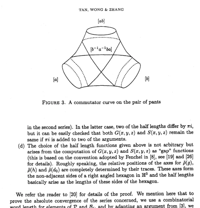
of [20] for details. Note that in this case, thecommutator $aba^{-1}b^{-1}$

of apair ofgenerators is anon-simple closed curve on the pair of pants,

as

shown in Figure 3, and that its trace tr$\rho(aba‘ 1b^{-1})>18$

.

4. The $\mathrm{S}\mathrm{L}(2, \mathrm{C})$ characters of a one-holed torus

The restriction of Theorem 2.1 to a torus with a cusp

was

the original identity obtained by $\mathrm{M}\mathrm{c}\mathrm{S}\mathrm{h}\mathrm{a}\mathrm{n}\mathrm{e}$in his thesis. The identity (2) restricted to a

one-cone

or

one-holed torus $T$

can

be regarded

as

generalizations ofthis original identity, and reinterpreted

as

an identity for representations (or

more

accurately, characters) of the one-holed torus group $\pi:=\pi_{1}(T)$ to $\mathrm{P}\mathrm{S}\mathrm{L}(2, \mathrm{R})$,

as we saw

in theprevious

sec-tion. It is naturalto ask how farthis result

can

be extended torepresentationsinto

$\mathrm{P}\mathrm{S}\mathrm{L}(2, \mathrm{C})$. Indeed one already has the extension to quasi-fuchsian representations

byBowditch, and the example given at the end oftheprevious section showed that

we

can extendthe identity to the

case

ofclassical Schottkyrepresentations, includ-ing those arisinclud-ing from

a

hyperbolic pair of pants. These, however, required

some

special properties including the discreteness of the representation, which seemed unnecessarilyrestrictive. For example, given a representation arising

as

the holo-nomy of

a

one-cone

hyperbolic torus withsay cone angle$\theta$ (whichis not necessarily

discrete),

one

would expect that for sufficiently small perturbations ofthe repre-sentation into $\mathrm{P}\mathrm{S}\mathrm{L}(2, \mathrm{C})$, the identity would still hold. This turns out to be true,

andin fact,

one

can

give verycomprehensive

answers

to the questions posedabove. For example,

we

can

obtain necessary and sufficient conditions for the generalized

$\mathrm{M}\mathrm{c}\mathrm{S}\mathrm{h}\mathrm{a}\mathrm{n}\mathrm{e}’ \mathrm{s}$identityto hold for

$\mathrm{r}\mathrm{e}\mathrm{p}\mathrm{r}\mathrm{e}\mathrm{v}\mathrm{e}\mathrm{n}\mathrm{t}\mathrm{a}\mathrm{t}\mathrm{i}\mathrm{o}\mathrm{n}\mathrm{s}/\mathrm{c}\mathrm{h}\mathrm{a}\mathrm{r}\mathrm{a}\mathrm{c}\mathrm{t}\mathrm{e}\mathrm{r}\mathrm{s}$of$\pi$ into $\mathrm{P}\mathrm{S}\mathrm{L}(2, \mathrm{C})$

.

For this, it turns out that Bowditch’s proof via $\mathrm{a}\mathrm{l}\mathrm{g}\mathrm{e}\mathrm{b}\mathrm{r}\mathrm{a}\mathrm{i}\mathrm{c}/\mathrm{c}\mathrm{o}\mathrm{m}\mathrm{b}\mathrm{i}\mathrm{n}\mathrm{a}\mathrm{t}\mathrm{i}\mathrm{o}\mathrm{r}\mathrm{i}\mathrm{a}\mathrm{l}$methods

are

extremely useful, and this is the approach

we use

andgeneralize in [22] and [21] to solve this problem. Another useful corollary of this method is that

we

are able to obtain various restricted and relative versions of the identity, the latter of which have geometric interpretations in terms of punctured torus bundles

over

the cir-cle, and in particular, allows

us

to prove identities for certain complete hyperbolic 3-manifolds obtained by hyperbolic Dehn surgery

on

hyperbolic punctured torus bundles.

For the rest of this section,

we

will first start with

some

basic definitions, then give

statements of some

of the main results, and finally list

some

of the key tech-niques and issues involved in the proofs ofthe results. We should

warn

the reader that the proofs

are

somewhat technical in

some

parts, details can be found in [6],

[22] and [21]. Note also that

we

shall be stating and proving results for represen-tations(characters) into $\mathrm{S}\mathrm{L}(2, \mathrm{C})$ instead of $\mathrm{P}\mathrm{S}\mathrm{L}(2, \mathrm{C})$

.

This makes

no

essential

difference since allrepresentations of$\pi$ into $\mathrm{P}\mathrm{S}\mathrm{L}(2, \mathrm{C})$

can

belifted to $\mathrm{S}\mathrm{L}(2, \mathrm{C})$

as

$\pi$ is free, and the identities obtained will be independent of the lift chosen, and

hence can be stated as identities for $\mathrm{P}\mathrm{S}\mathrm{L}(2, \mathrm{C})$ characters.

4.1. Basic Deflnitions. Let $T$be

a

one-holed torus and $\pi$ its fundamental

group

which is freely generated by two elements $X,$$\mathrm{Y}$ corresponding to simple closed

curves

on

$T$with geometric intersection number

one.

Definition

4.1.

The $\mathrm{S}\mathrm{L}(2, \mathrm{C})$ character variety

$\mathcal{X}:=\mathrm{H}\mathrm{o}\mathrm{m}(\pi, \mathrm{S}\mathrm{L}(2, \mathrm{C}))//\mathrm{S}\mathrm{L}(2, \mathrm{C})$

of$T$ istheset ofequivalence classes of representations $\rho:\pi\mapsto \mathrm{S}\mathrm{L}(2, \mathrm{C})$, where the

equivalence classes

are

obtained bytaking the closure of the orbits under conjuga-tion by $\mathrm{S}\mathrm{L}(2, \mathrm{C})$

.

TAN, WONG &ZHANG

The character variety stratifies into relative character varieties: for $\kappa\in \mathrm{C}$, the

$\kappa$-relative character variety ,

$\mathrm{V}_{\kappa}$ is the set of equivalence classes $[\rho]$ such that

tr$\rho(XYX^{-1}Y^{-1})=\kappa$

for one (and hence any) pair of generators $X,$$Y$ of $\pi$

.

Note that the

commutator

$XYX^{-1}Y^{-1}$ represents a peripheral

curve

in $T$

.

By classical results of IFIricke,

we

have the following identifications:

$\mathcal{X}\cong \mathrm{C}^{3}$,

$\mathcal{X}_{\hslash}\cong\{(x, y, z)\in \mathrm{C}^{3}|x^{2}+y^{2}+z^{2}-xyz-2=\kappa\}$,

where the identification isgiven by

$\iota$ : $[\rho]\vdasharrow(x, y, z):=(\mathrm{t}\mathrm{r}\rho(X), \mathrm{t}\mathrm{r}\rho(\mathrm{Y}),$

$\mathrm{t}\mathrm{r}\rho(X\mathrm{Y}))$,

for

a

fixed pair of generators $X,$$Y$ of $\pi$

.

The topology

on

X and

$\mathcal{X}_{\kappa}$ will be that

induced bythe above identifications.

The outer automorphism group of $\pi,$ $\mathrm{O}\mathrm{u}\mathrm{t}(\pi):=\mathrm{A}\mathrm{u}\mathrm{t}(\pi)/\mathrm{I}\mathrm{n}\mathrm{n}(\pi)\cong \mathrm{G}\mathrm{L}(2, \mathbb{Z})$ is

isomorphic to the mapping class group $\Gamma:=\pi_{0}(\mathrm{H}\mathrm{o}\mathrm{m}\mathrm{e}\mathrm{o}(T))$ of $T$ and acts

on

$\mathcal{X}$

,

preserving the trace of the commutator of

a

pair of generators, hence it also acts

on

$X_{\kappa}$

,

the action is given by

$\phi([\rho])=[\rho\circ\phi^{-1}])$

where $\phi\in \mathrm{O}\mathrm{u}\mathrm{t}(\pi)$ and $[\rho]\in \mathcal{X}$

or

,$\mathrm{V}_{\kappa}$ respectively. It is often convenient to

con-sider only the subgroup Out$(\pi)^{+}$ of “orientation-preserving” automorphisms,

cor-responding to the orientation-preserving homeomorphisms $\Gamma^{+}$ of $T$, which is iso-morphic to $\mathrm{S}\mathrm{L}(2, \mathrm{Z})$

.

The action of Out$(\pi)^{+}$ (respectively,

Out

$(\pi)$)

on

X and

$\mathrm{X}_{\kappa}$

is not effective, thekernel is $\{\pm I\}$

,

generatedby the elliptic involution of$T$

so

that

the effective action is by $\mathrm{P}\mathrm{S}\mathrm{L}(2, \mathrm{Z})$ (respectively, $\mathrm{P}\mathrm{G}\mathrm{L}(2,$$\mathrm{Z})$).

4.2. Simple curves; Pants graph.

Deflnition 4.2. We denote by $\mathscr{C}$ the set of free homotopy classes of nontrivial,

non-peripheral, unoriented simple closed

curves

on

$T$

.

Elements of$\mathscr{C}$

are

usually

denoted by $X,$$Y,$$Z,$$W$

.

The elements of$\mathscr{C}$correspond tocertainelements of$\pi/\sim$, where the equivalence $\mathrm{r}\mathrm{e}\mathrm{l}\mathrm{a}\mathrm{t}\mathrm{i}\mathrm{o}\mathrm{n}\sim \mathrm{i}\mathrm{s}$that, for

$g,$$h\in\pi,$ $g\sim h$ if and only if $g$ is conjugate to $h$or

$h^{-1}$

.

We

also denote the corresponding subset of$\pi/\sim \mathrm{b}\mathrm{y}\mathscr{C}$, thereshould be no confusion.

Deflnition

4.3.

The pants graph $\mathscr{C}(T)$ of $T$, is defined to be the graph whose

vertices

are

the elements of $\mathscr{C}$, and two vertices

are

joined by

an

edge if and only

ifthe corresponding

curves on

$T$ have geometric intersection number

one.

The mapping class group $\Gamma$ and Out$(\pi)$ act

on

$\mathscr{C}$ (respectively $\mathscr{C}(T)$)

$.2$We

can

realize $\mathscr{C}(T)$

as

the Farey $\mathrm{g}\mathrm{r}\mathrm{a}\mathrm{p}\mathrm{h}/\mathrm{t}\mathrm{r}\mathrm{i}\mathrm{a}\mathrm{n}\mathrm{g}\mathrm{u}\mathrm{l}\mathrm{a}\mathrm{t}\mathrm{i}\mathrm{o}\mathrm{n}$of the upper half plane

$\mathbb{H}$

so

that

$\mathscr{C}$ is identified with $\hat{\mathrm{Q}}:=\mathrm{Q}\cup\{\infty\}$, the action of

$\Gamma$ is

realized

by the action of

$\mathrm{P}\mathrm{G}\mathrm{L}(2, \mathrm{Z})$

on

the Farey graph. The projective lamination

space

$\mathscr{P}\mathscr{L}$ of$T$ is then

identified with $\hat{\mathrm{R}}:=\mathrm{R}\cup\{\infty\}$ and contains $\mathscr{C}$

as

the (dense) subset of rational

4.3. Bowditch $\mathrm{Q}$-conditions ($\mathrm{B}\mathrm{Q}$-conditions). We define a certain subspace

of$X$ which

we

will call theBowditch space. First note that for $[\rho]\in \mathcal{X}$ and$X\in \mathscr{C}$

,

tr$\rho(X)$ is well-defined.

Definition 4.4. The Bowditch space is the subset $X_{BQ}\subset X$ consisting of

charac-ters $[\rho]$ satisfying the following conditions (the Bowditch Q-conditions):

(1) tr$\rho(X)\not\in[-2,2]$ for all $X\in \mathscr{C}$;

(2) $|\mathrm{t}\mathrm{r}\rho(X)|\leq 2$ for only finitely many (possibly no) $X\in \mathscr{C}$

.

F’or

a

fixed $[\rho]\in X$ and $U\subset \mathscr{C}$,

we

say that the $\mathrm{B}\mathrm{Q}$-conditions

are

satisfied

on

$U$ for $[\rho]$ ifconditions (1) and (2) above hold for all $X\in U$

.

4.4. Statement ofresults for $\mathrm{S}\mathrm{L}(2, \mathrm{C})$ characters. We have the following

ex-tension and generalization ofTheorem 2.1 to characters in $X$

.

Theorem 4.5. (Theorems 2.2,

2.3

and Proposition 2.4 of [22]) (a) Bowditch space $X_{BQ}$ is open in the whole

character

space $X$

.

(b) The mapping class group $\Gamma$ acts properly discontinuously

on

$\mathcal{X}_{BQ}$

.

$f\mathrm{t}\iota$

rther-more, $X_{BQ}$ is the largest open subset

of

$X$

for

which this holds.

(c) For a character $[\rho]\in X_{BQ}\cap \mathcal{X}_{\kappa \mathrm{z}}$

$\sum_{X\in l}\log\frac{e^{\nu}+e^{l(\rho(X\rangle)}}{e^{-\nu}+e^{l(\rho(X))}}=\nu$ mod $2\pi i$, (14)

where $\nu=\cosh^{-1}(-\kappa/2)$, and the

sum

converges absolutely.

Remark 4.6.

(1) The (complex) length $l(\rho(X))$ is related to the trace

as

in equation (11).

(2)

We are

using the formula for $G(x, y, z)$ given in (6) for part (c), note that

there

are

no

$S(x, y_{)}z)$ terms since there is only

one

boundarycomp$\mathit{0}$nent.

(3) Inthe

case

when$\kappa=-2,$ $\nu=0$andallthe terms of(14)

are

identically

zero.

However, if

we

take the first order infinitesimals,

or

the formal derivative of (14) with respect to $\nu$ and evaluate at $\nu=0$,

we

get

$\sum_{X\in\vee}\frac{1}{1+e^{l(\rho(X))}}=\frac{1}{2}$, (15)

which is $\mathrm{M}\mathrm{c}\mathrm{S}\mathrm{h}\mathrm{a}\mathrm{n}\mathrm{e}’ \mathrm{s}$original identity in [12] for real type-preserving

char-acters, and also Bowditch’s generalization in [4] and [6] for type-preserving characters satisfying the BQ-conditions.

(4) When $\kappa=2$, which corresponds to the reducible characters, the identity

is also trivial. In this case, however, the Bowditch $\mathrm{Q}$-conditions

are never

satisfied,

see

[23].

(5) Parts (a) and (b) of the above

were

originally stated in [22] in terms of the relative character varieties $X_{\kappa}$

.

(6) $\nu$ is

a

specific choice ofhalfof the complex length of the peripheral

curve

on

$T$, note that the minus sign is crucial for the identity to hold.

4.5. Necessary and sufflcient conditions. Replacing condition (1) of the BQ-conditions by (1’) tr$\rho(X)\not\in(-2,2)$ for all $X\in \mathscr{C}$,

we

get the extended Bowditch

TAN, WONG& ZHANG

Theorem

4.7.

(Theorem 1.5 of [21]) For $[\rho]\in \mathcal{X}_{f}$ the identity (14)

of

Theorem

4.5(c) holds (with absolute

convergence

_of

the sum)

_if

and only

_if

$[\rho]$ lies in the

extended Bowditch space $\hat{X}_{B\mathrm{Q}}$.

The aboveresult gives acomplete

answer

to the question of when the generalized

$\mathrm{M}\mathrm{c}\mathrm{S}\mathrm{h}\mathrm{a}\mathrm{n}\mathrm{e}’ \mathrm{s}$identity holds for $\mathrm{S}\mathrm{L}(2, \mathrm{C})$ characters of$T$

.

4.6. $\mathrm{M}\mathrm{c}\mathrm{S}\mathrm{h}\mathrm{a}\mathrm{n}\mathrm{e}$-Bowditch identities for punctured torus bundles. We next

consider further variations of the $\mathrm{M}\mathrm{c}\mathrm{S}\mathrm{h}\mathrm{a}\mathrm{n}\mathrm{e}$

-Bowditch

identities. Recall that $\theta\in$

$\mathrm{O}\mathrm{u}\mathrm{t}(\pi)\cong\Gamma$ acts

on

X where the action is given by

$\theta([\rho])=[\rho 0\theta^{-1}]$

.

Supposethat $[\rho]\in \mathcal{X}$ is

stabilized

by

an

Anosov element

$\theta\in\Gamma^{+}$ (this corresponds

to

a

hyperbolic element if we identify $\Gamma^{+}$ with $\mathrm{S}\mathrm{L}(2, \mathrm{Z}))$, that is, $\theta([\rho])=[\rho]$

.

We

can

associate to this

a

representation of $\pi_{1}(M)$ into $\mathrm{S}\mathrm{L}(2, \mathrm{C})$

,

where $M$ is a

punctured torus bundle

over

the circle, with monodromy $\theta$

.

The restriction of

the representation to the fibre is $[\rho]$

.

We

can

find

a

specific lift of

$\theta$ to $\mathrm{A}\mathrm{u}\mathrm{t}(\pi)$

which corresponds to choosing a specific longitudeoftheboundary torus of$M$ (see

[5]

or

[22] for details). So fixing a representation $\rho$ in the class

$[\rho]$

,

there exists

$A\in \mathrm{S}\mathrm{L}(2, \mathrm{C})$ such that for all $\alpha\in\pi$

,

$\theta(\rho)(\alpha)=A\cdot\rho(\alpha)\cdot A^{-1}$

.

Note that tr$A$ is independent of the choice of $\rho$ in the conjugacy class

$[\rho]$

.

Note

also that tr$\rho(X)$ is well-defined

on

the equivalence classes [X] $\in \mathscr{C}/(\theta\rangle$

.

Suppose

further that $[\rho]$ satisfies the relative Bowditch $\mathrm{Q}$-conditions

on

$\mathscr{C}/(\theta\rangle$, that is,

(1) tr$\rho(X)\not\in[-2,2]$ for all $[X]\in \mathscr{C}/\langle\theta\rangle$;

(2) $|\mathrm{t}\mathrm{r}\rho(X)|\leq 2$ for only finitely many $[X]\in \mathscr{C}/\langle\theta\rangle$

.

Using the identification of$\Gamma^{+}$ with $\mathrm{S}\mathrm{L}(2, \mathrm{Z})$ and$\mathscr{C}$ with $\hat{\mathrm{Q}}\subset\hat{\mathrm{R}}\cong \mathit{9}\mathscr{L}$ in

\S 4.2,

we

get that the repelling and attracting fixed points of$\theta,$ _{$\mu_{-},$}$\mu+\in \mathrm{f}\mathscr{L}$ partition $\mathscr{C}$

into two subsets $\mathscr{C}_{L}\coprod \mathscr{C}_{R}$ which

are

invariant under the action of

$\theta$

.

We have the

following generalizations of the $\mathrm{M}\mathrm{c}\mathrm{S}\mathrm{h}\mathrm{a}\mathrm{n}\mathrm{e}$-Bowditch identities:

Theorem 4.8. (Theorems 5.6 and

5.9

of [22]) Suppose that $[\rho]$ is stabilized by an

Anosov element $\theta\in\Gamma^{+}$ and

satisfies

the relative

Bowditch

$Q$-conditions

as

stated

above. Then

$\sum_{[X]\in l/\langle\theta)}\log\frac{e^{\nu}+e^{l(\rho(X))}}{e^{-\nu}+e^{l(\rho(X))}}=0$ mod

$2\pi i$, (16)

and

$\sum_{[X]\in l\iota/\langle\theta\rangle}\log\frac{e^{\nu}+e^{l(\rho(X))}}{e^{-\nu}+e^{l(\rho(X))}}=\pm l(A)$ mod

$2\pi i$, (17)

where the

sums

converge absolutely; and$l(A)$ is the complex length

of

the

conjugat-$ing$ element $A$ corresponding to $\theta$

as

described above, and the sign in (17) depends

only

on

our

choice

_of

orientations.

Remark

4.9.

Fortype-preservingcharacters$(\kappa=-2)$,the resultisduetoBowditch

[5], where the summands of (16) and (17) should be replaced appropriately

as

in Remark 4.6(3) by the summands of$\mathrm{M}\mathrm{c}\mathrm{S}\mathrm{h}\mathrm{a}\mathrm{n}\mathrm{e}’ \mathrm{s}$original identity, and $l(A)$ in (17)

volume hyperbolic structure. There are also similar identities in the

case

where $\theta$

is reducible, that is, corresponds to aparabolic element of$\mathrm{S}\mathrm{L}(2, \mathrm{Z})$, see [21].

The above result has applications to closed hyperbolic 3-manifolds. As before, let $M$be

an

orientable 3-manifoldwhich fibers overthecircle, withthe fiber

a

once-punctured torus, $T$andsuppose that the monodromy $\theta$of$M$ is Anosov. By results

of Thurston,

see

[25] and [24], $M$ has a complete finite-volume hyperbolic

struc-ture with a single cusp, which

can

in turn be deformed to incomplete hyperbolic structures,

on

which hyperbolic Dehn surgery

can

be performed to obtain complete hyperbolic manifolds without cusps. Restricting the holonomy representation to the fiber gives

us

characters which

are

stabilized by $\theta$, and in the complete case,

the relativeBowditch $\mathrm{Q}$-conditions

are

satisfied (see [5]). For smalldeformationsof

the complete structuretoincomplete structures, the relative$\mathrm{B}\mathrm{Q}$-conditions

are

still

satisfied sincethese

are

open conditions (see [22]). Theidentities can beinterpreted

as

series identities for these (in)complete structures, involving the complex lengths ofcertain geodesicscorresponding to the homotopy classesofessential simpleclosed

curves on

the fiber. The quantity $\nu$

can

be interpreted

as

halfthe complex$1\mathrm{e}\mathrm{i}_{1}\mathrm{g}\mathrm{t}\mathrm{h}$of

the meridian of the boundary torus, and $l(A)$

as

the complex length of

a

(suitably

chosen) longitude of the boundary torus. In particular, the identity

can

be

inter-preted

as

an

identity for the closed hyperbolic 3-manifolds obtained by hyperbolic Dehn surgery

on

the original complete manifold, if the Dehn surgery invariants

are

sufficiently close to $\infty$

.

One questionwhich arises is whether the identity holds for all closed hyperbolic 3-manifolds obtained by hyperbolic Dehn surgery

on a

hyperbolicpunctured torus bundle

over

the circle. The openness of the relative $\mathrm{B}\mathrm{Q}$-conditions

ensures

that

this is true for almost all such manifolds (except for possibly

a

finite number of exceptions). Another question arising is whether

a

similar result holds in the

case

ofhyperbolic Dehn surgery

on

punctured surface bundles,

as

studied by Akiyoshi, Miyachi and Sakuma [2].

4.7. Key points used in the proofs. The combinatorial structure of $\mathscr{C}(T)$

as

well

as

the Fricke trace relation which

can

be interpreted

as

an edge relation play fundamental roles which

we

sketch $\mathrm{h}e\mathrm{r}\mathrm{e}$

.

Recall that $\mathscr{C}(T)$ has the structure of the Farey tessellation, and the set of

vertices $\mathscr{C}$ can be identified with Q. The dual graph $\Sigma$ to _{$\mathscr{C}(T)$} is a trivalent tree

whose complementary regions

can

be identified with the vertices of$\mathscr{C}(T)$

.

Denote

by $V(\Sigma),$ $E(\Sigma),\vec{E}(\Sigma)$ and $\Omega(\Sigma)$ the sets of vertices, edges, directed edges and

complementary regions of $\Sigma$ respectively. Call (X,Y) $\in \mathscr{C}\cross \mathscr{C}$

a

generating pair

if $X$ and $\mathrm{Y}$

are

connected by

an

edge in $\mathscr{C}(T)$, and $(X, Y, Z)\in \mathscr{C}\cross \mathscr{C}\cross \mathscr{C}$ a

generating triple if $X,$$Y$

and

$Z$

are

the vertices of

a

triangle in $\mathscr{C}(T)$

.

Generating

pairs correspond to edges of $\Sigma$ and generating triples correspond to vertices of

$\Sigma$

.

More specifically, to

an

edge _$e$ of $\Sigma$,

we

write $e=(X, Y;Z, Z’)$ if (X,$Y$)

corresponds to $e$ and (X,$Y,$ $Z$), $(X, Y, Z’)$

are

generating triples. Similarly,

we

use $earrow=(X, \mathrm{Y};Zarrow Z’)$ to indicate that the directed edge $e\mathrm{p}\mathrm{o}\mathrm{i}arrow \mathrm{n}\mathrm{t}\mathrm{s}\mathrm{h}\mathrm{o}\mathrm{m}Z$ to

$Z$‘,

see

Figure 5, where

we

have drawn part of $\Sigma$, and used the identification of

$\Omega(\Sigma)$ with $\mathscr{C}$. Denote by $-e\mathrm{t}\mathrm{h}arrow \mathrm{e}$ directed edge with the opposite direction to

$earrow$. For $earrow=$ $(X, \mathrm{Y};Zarrow Z‘)$, we define Tai1$(e)\neg$, the tail of $e\mathrm{t}\mathrm{o}arrow$ be the subset of

$\mathscr{C}$ in the interval between $X$ and $\mathrm{Y}$ (inclusive) which contains $Z$. In particular,

TAN, WONG&ZHANG

For each character $[\rho]\in X_{\kappa}$, by taking the trace function,

we

obtain a trace map

$\phi$ : $\mathscr{C}arrow \mathrm{C}$ where $\phi(X)=\mathrm{t}\mathrm{r}\rho(X)$

.

(We call it

a

generalized Markoff map in [22] following [6].)

Henceforth, for

a

fixedtrace map $\phi$

, we

adopt the convention of using the lower

case

letters to represent the values of $\phi$, that is, $\phi(X)=x,$ $\emptyset(Y)=y$, etc. Then

$\phi$ satisfies the following vertex and edge relations, arising from the Fricke trace

identities:

Vertex relation. For everygenerating triple (X,$\mathrm{Y},$$Z$),

$x^{2}+y^{2}+z^{2}-xyz-\kappa-2=0$

.

(18)

Edge relation. For every edge $e=(X, Y;Z, Z’)$,

$z+z’=xy$

.

(19)

It turns outthat the edgerelationis

more fundamental

than the vertex relation. To start with,

one can

show easily that if the edge relation is satisfied for all edges, than the vertex relation propagates along the edges to

cover

the entire tree

$\Sigma$

.

Secondly, $\phi$ is completely determined by its values

on

any generating triple

(X,$\mathrm{Y},$$Z$) by successively applying theedge relation (19).

Each $[\rho]\in \mathcal{X}$ (equivalently, the induced trace map $\phi$ on $\mathscr{C}$) determines

a

map $f$ : $E(\Sigma)arrow\vec{E}(\Sigma)$, where each edge $e$is assigned adirection or flow $\mathrm{h}\mathrm{o}\mathrm{m}$the larger

absolute value to the smaller one, that is,

$f(e)=e=arrow(X, \mathrm{Y};Zarrow Z’)$

if $|z|\geq|z’|$

.

There is

some

ambiguity when $|z|=|z’|$ in which

case we can

assign

either direction.

This ambiguity does not affect the large

scale

behavior of$f(E(\Sigma))$,

except in

some

very special trivial

cases.

We then have the following elementary

but important results (see [22] for proofs). For the purposes ofour discussion,

we

fix $[\rho]\in X_{\kappa}$ where $\kappa\neq 2$ ($[\rho]$ is not reducible), with corresponding trace map $\phi$

.

Proposition 4.10.

_If

(X,$Y,$$Z$) is

a

generating triple corresponding to the vertex $v\in V(\Sigma)$ and $f(e)$ points away

from

$v$

for

at least two

of

the edges adjacent to $v$

,

then $\min(|x|, |y|, |z|)\leq 2$

.

Lemma 4.11. (Bowditch [6]) For all $K\geq 2,$ $\mathscr{C}(K):=\{X\in \mathscr{C}|\phi(X)\leq K\}$

is connected, that is, the subgraph

of

$\mathscr{C}(T)$ spanned by $\mathscr{C}(K)$ is connected. $In$

panicular, $\mathscr{C}(2)$ is connected.

The above

can

be regarded

as a

quasi-convexity result, namely, for any $K\geq 2$,

for any $X,$$Y\in \mathscr{C}(K)$, the geodesic in $\mathscr{C}(T)$ joining $X$ to $Y$ is

a

bounded

distance $\mathrm{h}\mathrm{o}\mathrm{m}$ the subgraphin _{$\mathscr{C}(T)$} spannedby _{$\mathscr{C}(K)$}

.

Proposition 4.12. Suppose that $X\in \mathscr{C}$ and$Y$ , $n\in \mathrm{Z}$

are

the neighbors

of

$X$, in

cyclical order.

(a)

_If

$x\not\in[-2,2]\cup\{\pm\sqrt{\kappa+2}\}$, then $\lim_{narrow\pm\infty}|y_{n}|=\infty$ with exponential growth in $|n|$

.

(b)

_If

$x=\pm 2$ and $\kappa\neq 2_{J}$ then $\lim_{narrow\pm\infty}|y_{n}|=\infty$ with lineargrowth in $|n|$

.

The proof of Theorem 4.5 now proceeds

as

follows:

First

we

show that the $\mathrm{B}\mathrm{Q}$-conditions are open conditions. This is achieved by

showing that the conditions

are

controlled by a finite subtree of $\Sigma$; the proof is