An exact algorithm for the budget-constrained multiple knapsack problem (Decision Making Processes under Uncertainty and Ambiguity)

An

exact

algorithm for the budget-constrained

multiple knapsack problem

Department of

Computer

Science,

The National

Defense

Academy

Yokosuka,

_{Kanagawa 239-8686, Japan}

Byungjun

You,

_{Takeo Yamada}

{g48095,

yamada}@nda.ac.jp

1

Introduction

This

paper

isconcemed with

a

variationof the multiple knapsack problem (MKP) [5, 6],where

we

are

given

a

setof $n$ items _{$N=\{1,2, \ldots, n\}$} to be packed into $m$ possible knapsacks $M=\{1,2, \ldots, m\}$_. As in ordinary

MKP,by $w_{j}$ and $p_{j}$ wedenote the weight and profit of item$j\in N$ respectively, and the capacityof knapsack

$i\in M$ is$c_{j}$. However,a fixedcost$f_{i}$ is imposed if

we use

knapsack$i$, andknapsacks

are

freely available within

afixed budget $B$

.

The problem istodetermine thesetof knapsacks_tobe employed

as

wellas tofill theadopted knapsacks with items such thatthecapacity constraintsareall satisfied and thetotal profit is maximized. Let $y_{i}$ and$x_{ij}$be the decision variables such that$y_{i}=1$ if

we use

knapsack$i$, and_{$y_{i}=0$}otherwise. Also,

$x_{ij}=1$ if item $j$ is put into knapsack $i$, and

$x_{ij}=0$ otherwise. Then, the problem is formulated

as

_{the following}

budget-constrained multiple knapsackproblem.

BCMKP:

maximize $\sum_{i=1}^{m}\sum_{j=1}^{n}p_{j^{X}ij}$ (1)

subjectto $\sum_{j=1}^{n}w_{j}x_{ij}\leq c;y_{i}$, $i\in M$, (2)

$\sum_{i=1}^{m}x_{ij}\leq 1$, $j\in N$, (3)

$\sum_{i=1}^{m}f_{i}y_{i}\leq B$, (4)

$x_{ij},$ $y_{i}\in\{0,1\}$, $i\in M,j\in N$. (5)

Throughoutthe paper we

assume

the following.

$A_{1}$. Problem data

$w_{j},$ $p_{j}(j\in N),$ $c_{i},$ $f_{i}(i\in M)$and $B$are allpositive integers.

$A_{2}$. Items

are

arrangedinnon-increasingorderof profitperweight, i.e.,

$p_{1}/w_{1}\geq p_{2}/w_{2}\geq\ldots\geq p_{n}/w_{n}$. ₍₆₎

A3.

Knapsacks

are

numberedin non-increasingorderofcapacitypercost,i.e.,

$c_{1}f_{1}\geq c_{2}f_{2}\geq\ldots\geq c_{m}’ f_{m}$. ₍₇₎

BCMKP is NP-hard [3],_{since the special}

_case

_{of free knapsacks}$(f_{i}\equiv 0, \forall i\in M)$ is simplyanMKP which

is already NP-hard. Since BCMKP isalinear0-1 programmingproblem, small instances

can

besolved using MIP(mixedintegerprogramming) solvers. In thisarticle,

we

present

an

algorithmthat solves largerBCMKPs

2

Upper bound

Thissectionderives

an

upperboundby applyingtheLagrangian relaxation[2]toBCMKP. Withnonnegative

multipliers $\lambda=(\lambda_{i})\in R^{m}$ and$\mu\in R$ associated with (2) and (4) respectively, theLagrangian relaxation to

BCMKPis LBCMKP$(\lambda,\mu)$

:

maximize $\sum_{i=1}^{m}\sum_{j=1}^{n}(p_{j}-\lambda_{i}w_{j})x_{ij}+\sum_{i=1}^{m}(\lambda_{i}c_{i}-\mu f_{i})y_{i}+\mu B$ (8)

subject to (3), (5).

For$\lambda\geq 0,$$\mu\geq 0$, let$\overline{z}(\lambda,\mu)$ denote the optimal objective valuetoLBCMKP$(\lambda,\mu)$

.

Then, it is easily proved

that$\overline{z}(\lambda,\mu)$gives an upperboundto BCMKP, and$\overline{z}(\lambda,\mu)$is

a

piecewise linear and

convex

function of$\lambda$and

$\mu$. Moreover,ifweconsider the Lagrangian dual

minimize $\overline{z}(\lambda,\mu)$ subjectto $\lambda\geq 0,\mu\geq 0$,

we

have thefollowing.

Theorem1 Thereexistsanoptimalsolution$\lambda^{\dagger}=(\lambda_{i}^{\dagger})$ tothe Lagrangian dual suchthat$\lambda_{1}^{\dagger}=\lambda_{2}^{\dagger}=\ldots=\lambda_{m}^{\dagger}(\equiv$

$\lambda^{\dagger})$.

Proof. Fora fixed $\lambda=(\lambda_{i})\geq 0$, let $k$ $:= \arg\min_{i\in M}\{\lambda_{i}\}$

.

Then, since $p_{j}-\lambda_{i}w_{j}\leq p_{j}-\lambda_{k}w_{j}$ for all $i\in M$

and$j\in N$, the objective function (8) is maximized by setting $x_{ij}=1$ if and only if$i=k$ and$p_{j}-\lambda_{k}w_{j}>0$

.

Similarly,$y_{i}=1$ if and only if$\lambda_{i}c_{i}-\mu f_{i}>0$, and

we

obtain

$\overline{z}(\lambda,\mu)=\sum_{j=1}^{n}(p_{j}-\lambda_{k}w_{j})^{+}+\sum_{i=1}^{m}(\lambda_{i}c_{i}-\mu f_{i})^{+}+\mu B$, (9)

where $(\cdot)^{+}$ _{$:= \max\{\cdot, 0\}$}

.

Here, we note that $(\lambda_{i}c_{i}-\mu f_{i})^{+}$ is monotonically non-decreasing with respect to $\lambda_{i}(i\neq k)$. Thus, under thecondition$\lambda_{i}\geq\lambda_{k},$ (9) is minimizedat$\lambda_{i}\equiv\lambda_{k}(i\in M)$. ₁

From thistheorem, it sufficestoconsiderthe

case

of$\lambda_{i}\equiv\lambda(\forall i\in M)$,andthus$\overline{z}(\lambda,\mu)$ is rewritten

as

$\overline{z}(\lambda,\mu)=(C_{t}-W_{s})\lambda+(B-F_{t})\mu+P_{s}$. (10)

Here $s$ and $t$

are

the critical valuesdefined

as

$s$ $:= \max\{j|p_{j}-\lambda w_{j}\geq 0\}$ and $t$ _{$:= \max\{i|\lambda c_{i}-\mu f_{i}\geq 0\}$}

respectively, and $W_{s}$ is the accumulated weight given by$W_{s}$ $:= \sum_{j=1}^{s}w_{j}$

.

$P_{s},$$C_{t}$ and$F_{t}$areanalogously defined

for $(p_{j}),$ $(c_{i})$ and $(f_{i})$, respectively. Forafixed$\mu\geq 0,$ (10) isa piecewise linear function of$\lambda$, and its gradient

changes from$C_{t}-W_{s}$to $C_{t}-W_{s-1}$ as$\lambda$increases from$p_{t}w_{s}-0$to$p_{s}w_{s}+0$. Similarly, the gradientincreases

from$C_{t-1}-W_{s}$to $C_{t}-W_{s}$ at$\lambda=(f_{t}c_{t})\mu$

.

Thus,

we

obtaintheoptimal$\lambda$as

$\lambda^{\dagger}(\mu)=\{\begin{array}{ll}p_{s}’ w_{s}, if W_{s-1}\leq C_{f}\leq W_{s},(f_{t}’ c_{t})\mu, if C_{t-1}\leq W_{s}\leq C_{t}.\end{array}$ (11)

Putting this into (10), $\overline{z}(\lambda^{\dagger}(\mu),\mu)$ is also piecewise linear with respect to

$\mu$, and by bisection method

we

obtain

an

optimal$\mu^{\dagger}$ and $\lambda^{\dagger}$

$:=\lambda^{\dagger}(\mu\dagger)$,andcorrespondingly

an

upperbound$\overline{z}=\overline{z}(\lambda^{\dagger}(\mu^{\dagger}),\mu^{\dagger})$. Let

us

introduce thethresholds

as

$\theta_{j}:=p_{j}-\lambda^{\dagger}w_{j}$, $\eta;:=\lambda^{\dagger}c_{i}-\mu^{\dagger}f_{i}$. (12) Then, from(9)theLagrangianupperboundis givenas

$\overline{z};=\overline{z}(\lambda^{\dagger},\mu^{\dagger})=\sum_{j\in N}\theta_{j}^{+}+\sum_{i\in M}\eta_{i}^{+}+\mu^{\dagger}$

3

Problem reduction

Assume that we have the optimal Lagrangian multipliers $\lambda^{\dagger}$

and$\mu^{\dagger}$ with the corresponding

upper

bound$\overline{z}$

givenby (13),

as

well

as a

lowerbound$\underline{z}$ obtained by

some

heuristic algorithmes. Let

$\delta$ be either$0$

or

1, and

we

introduce $P(y_{k}=\delta)$

as

the subproblem ofBCMKP with $y_{k}$ fixed at $\delta$. $\overline{P}(y_{k}=\delta)$ denotes theLagrangian

relaxationof$P(y_{k}=\delta)$using the optimal $\lambda^{\dagger}$

and$\mu^{\dagger}$ in (8). Thatis,

$\overline{P}(y_{k}=\delta)$;

maximize $\sum_{j=1}^{n}\theta_{j}x_{j}+\sum_{i=1}^{m}\eta_{i}y_{i}+\mu^{\dagger}B$ (14)

subjectto $x_{j},y_{i}\in\{0,1\},$$\forall j\in N,$$\forall i\in M,y_{k}=\delta$, (15)

where

we

introduce a new 0-1 variable$x_{j}$definedby $x_{j}= \sum_{i=1}^{m}x_{ij}$

.

Let $(x^{*},y^{*})$ be

an

optimal solution to BCMKP with _{$x^{*}=(x_{ij}^{*})$} and $y^{*}=(y_{i}^{*})$

.

Then, the following is

immediate.

Theorem2 (Peggingofknapsacks)Forevery$k\in M$,

(i) If$\eta_{k}>0$and$\overline{z}-\underline{z}\leq\eta_{k}\Rightarrow y_{k}^{*}=1$,

(ii) If$\eta_{k}<0$and$\overline{z}-z\sim\leq-\eta_{k}\Rightarrow y_{k}^{*}=0$

.

Proof. (i)Note that theoptimal objective value to$\overline{P}(y_{k}=\delta)$ is _{$\overline{z}(Jk=\delta)$}

$:= \sum_{j\in N}\theta_{j}^{+}+\sum_{i*k}’\epsilon M\eta_{i}^{+}+\mu^{\dagger}B+\eta_{k}\delta$

.

Then,comparingthis with (13)

we

have$\overline{z}(Jk=0)=\overline{z}-\eta_{k}\leq\underline{z}$, which implies$y_{k}^{*}=1$ in anyoptimal solution.

(ii)_{is similarly proved. 1}

Applying Theorem 2, the knapsacks

are

classifiedintothreedisjoint subsets$K_{0}$ _{$:=\{i\in M|y_{i}^{*}=0\},$} $K_{1}$ $:=\{i\in$

$M|y_{i}^{*}=1\}$ and theremaining $M\backslash (K_{0}\cup K_{1})$

.

Knapsack$i\in K_{0}$ is

never

used, while$i\in K_{1}$ is always used inany

optimal solutiontoBCMKP.

Similarly, we

can

derivea peggingtheoremforitems, andapplying thisclassifyitems into the disjointsets $I_{0}$ _{$:=\{j\in N|x_{j}^{*}=0\},$} $I_{1}$ _{$:=\{j\in N|x_{j}^{*}=1\}$} and$N\backslash (I_{0}\cup I_{1})$. Removing $K_{0}$ and$I_{0}$, BCMKP is reduced(often

significantly) insize. In whatfollows,we

assume

that thesearealreadydone, and thus$K_{0}=I_{0}=\emptyset$.

4

A branch-and-bound algorithm

A characteristic feature of the branch-and-bound algorithmto begiven below is that branchings

are

made

withrespect tovariables$(y_{i})$irrespectiveto$(x_{ij})$,andthelatteris determined onlyateach terminalsubproblems.

Toconstmct such

a

branch-and-bound algorithm,

we

introduce

a

subproblem ofBCMKP

as

follows. Let $F_{0}$

and$F_{1}$ betwosubsetsof$M$such that

$K_{0}\subseteq F_{0},$ $K_{1}\subseteq F_{1}$ and$F_{0}\cap F_{1}=\emptyset$.

Theserepresent the setsof knapsacks whicharefixedat$0$and 1,respectively. We considerthefollowing.

$P(F_{0}, F_{1})$: maximize(1) subjectto (2)$-(5)$,and

$y_{i}=0,$ $\vee i\in F_{0}$, $y_{i}=1,$ $\forall i\in F_{1}$

.

(16)

Usingtheoptimal $\lambda^{\dagger}$

and$\mu^{\dagger}$ obtainedin Section 2, theLagrangian relaxationtothis problemis

$\overline{P}(F_{0}, F_{1})$; maximize(14) subjectto_{$x_{j},y_{i}\in\{0,1\},$}$\forall j\in N,$ $\forall i\in M$and (16).

Let $z^{*}(F_{0}, F_{1})$ and $\overline{z}(F_{0}, F_{1})$ be the optimal objective values to these problems, respectively. Clearly, $\overline{z}(F_{0}, F_{1})$gives

an

upperboundto$z^{*}(F_{0}, F_{1})$, i.e.,$z^{*}(F_{0}, F_{1})\leq\overline{z}(F_{0}, F_{1})$; and

we

have

where $U$ _{$:=M\backslash (F_{0}\cup F_{1})$} is the _{set of unfixed knapsacks.}

Then, if

we

have

an

incumbent lower bound $\underline{z}$

satisfying$\overline{z}(F_{0}, F_{1})\leq\underline{z}$,

we

canterminate subproblem_{$P(F_{0}, F_{1})$}.

Other conditions for pruning subproblems

are

feasibility and dominance. First ofall, if the total cost of acceptedknapsacks is larger than thebudget, i.e., if$\sum_{i\in F_{1}}f_{i}>B,$ $P(F_{0}, F_{1})$is infeasible,and thus terminated.

Next, if

we

have knapsacks $(i_{0}, i_{1})\in F_{0}\cross F_{1}$ such that

$c_{i_{0}}\geq c_{i_{1}}$ and $f_{i_{0}}\leq f_{i_{}},$ $P(F_{0}, F_{1})$ is again terminated.

Indeed, ifsuch a pair $(i_{0}, i_{1})$ exists,

we

can define a subproblem

$P(F_{0}’, F_{1}’)$ by exchanging the role ofthese

knapsacks

as

$F_{0}’$ $:=F_{0}\cup\{i_{1}\}\backslash \{i_{0}\}$ and $F_{1}’$ $:=F_{1}\cup\{i_{0}\}\backslash \{i_{1}\}$. Then, $P(F_{0}, F_{1})$is dominated by$P(F’F’)$_, since

all thefeasible solutionsof$P(F_{0}, F_{1})$

are

feasibleto_{$P(F_{0}’, F_{1}’)$.}

$0$’ ₁

If$P(F_{0}, F_{1})$ is not terminated by any _{of these criteria, and in addition if}

$U$ is non-empty, we pick up

a

knapsack $i\in U$ _{and generate two subproblems of}$P(F_{0}, F_{1})$ as $P(F_{0}\cup\{i\}, F_{1})$ and $P(F_{0}, F_{1}\cup\{i\})$

.

On the

otherhand, if $U=\emptyset,$ $P(F_{0}, F_{1})$ is

a

terminal subproblem. _{Here, $P(F_{0}, F_{1})$ is}

an

_{MKP with}

respect to theset

of knapsacks $F_{1}$. An upperboundtothis subproblem can

be obtainedby solving thefollowing 0-1 knapsack

problem, which is obtainedbyreplacingthe set ofknapsacks withasingle knapsack of capacity$\sum_{i\in F_{1}}c_{i}$. Let

the break item$b$be given by_{$b= \min\{j;\sum_{i=1}^{j}w_{i}\leq\sum_{i\in F_{1}}c_{i}\}$}

. Linear relaxation gives an upperbound,calledthe

Dantzigbound, tothis problem

as

$\overline{z}_{term}(F_{0}, F_{1})=\lfloor P_{b-1}+\frac{c_{b}}{w_{b}}(\sum_{i\in F_{1}}c;-W_{b-1})\rfloor$, (18)

and if$\overline{z}_{te}(F_{0}, F_{1})\leq\underline{z},$$P(F_{0}, F_{1})$ is also terminated. Otherwise,

we

_{solve this MKP by calling MULKNAP}

[8], and obtain the optimal$z^{*}(F_{0}, F_{1})$

.

If this is better than the incumbent lower bound

$\underline{z}$,

we

update this

as

$\underline{z}arrow z^{*}(F_{0}, F_{1})$

.

Then,

_{we can}

_construct

_{a branch-and-bound}

_{algorithm to solve} $P(F_{0}, F_{1})$

as a

recursive procedure. The

algorithmstarts with the initial lower bound$\underline{z}$ and $(F_{0}, F_{1})$ $:=(K_{0}, K_{1})$, and in termination produces

an

opti-mal solution to BCMKP. However, inimplementing thebranch-and-bound algorithm,

we

have to specify the

strategy for the choice of thebranching knapsack $i$, as well as the method to traverse the

branch-and-bound

tree. As for the branching knapsack, underassumption A3, we pick up the unfixed knapsack of the smallest

index,i.e.,$i:= \min\{k|k\in U\}$, andcall$P(F_{0}, F_{1}\cup\{i\})$recursively before calling$P(F_{0}\cup\{i\}, F_{1})$

.

This

means

that

5

Numerical

experiments

We evaluate theperformance ofthe branch-and-bound algorithm oftheprevious section througha series of numerical experiments. We implement thealgorithmin ANSI$C$language and conductcomputation

on an

Dell

Precision T7400 workstation (CPU: XeonX5482$Quad- Core\cross 2,3.20GHz$).

5.1

Design

of

experiments

Instances areprepared within the rangeof$200\leq n\leq 160000$_and $5\leq m\leq 150$ according _to the following

scheme. The weight$w_{j}$ is distributed uniformly random

over

the integer interval [10, 1000], and profit$p_{j}$ is

relatedto $w_{j}$in the followingway.

.

Uncorrelated

case

(UNCOR): uniformlyrandomover[10, 1000], independent of$w_{j}$.

.

Weaklycorrelated

case

(WEAK):unifonnly random

over

$[w_{j}, w_{j}+200]$.

.

Stronglycorrelatedcase (STRONG):$p_{j}$ $:=w_{j}+20$

Knapsack capacity $c_{i}$ is determined by $c_{i}=\lfloor 5\alpha)n\cdot\alpha\cdot\xi_{i}\rfloor$, where $(\xi_{i})$ is uniformly distributed

over

the simplex$\{(\xi_{1}, \ldots,\xi_{m})|\sum_{i=1}^{m}\xi_{i}=1,\xi_{i}\geq 0\}$,and$\alpha$is

a

parameter tocontrol theratioofitems that

can

be accepted intotheknapsacks. Sinceaverageweight of items is approximately500,$\alpha=0.50$

means

that aboutahalf of all theitemscan be accommodated in the knapsacks. Knapsackcost is given by$f_{i}$ _{$:=\rho;c_{i}$}, where$\rho_{i}$ is uniformly random over[0.5, 1.5], and thebudget $B$is chosenas $B= \beta\sum_{i=1}^{m}f_{i}$. Here$\beta$ is anotherparameterthatcontrols

theratio of the budget$B$

over

the totalcostof knapsacks.

5.2

Comparison against

MIP

solvers

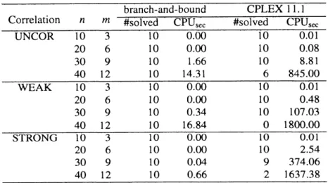
Table 1: Comparison againstMIPsolvers.

$\overline{\frac{Corre1ationnm\frac{branch- and- bou.ndCPLEX11.1}{\#so1v_{10000100.01}edCPU_{\sec}}}{UNCOR103}}$

#solved

$CPU_{\sec}$

20 6 10 $0.(K)$ 10 0.08 30 9 10 1.66 10 8.81 40 12 10 14.31 6845.00

$\overline{WEAK103100.00100.01}$

20 6 10 0.00 10 0.48 30 9 10 0.34 10 107.03

$\frac{40121016..84}{STRONG10310000100.01}$

$0$

1800.00

20 6 10 0.00 10 2.54 30 9 10 0.04 9 374.06 40 12 10 0.66 2 1637.38

Table 1 summarizes thecomputationof small instanceswith parameters$\alpha=0.5$ and_{$\beta=0.6,$$n=10\sim 40$}

and$m=3\sim 12$ using MIP solver CPLEX 11.1 [4] and thebranch-and-bound method of section 4. For each correlation type and values of$n$ and $m,$ $10$ random instances

are

generated and solved. Here shown

are

the

number of instances solved to optimality (#solved) within a fixed CPU time, and the average CPU time in

seconds. We set the time-limit ofcomputation at 1800CPU seconds, and ifcomputation is truncated due to

this time-limit,the CPU time for this instance is interpreted

as

1800seconds in computingaverages.

From Table 1

we see

that commercial solversare able to solveonly very small instances within the

5.3

Large

instances

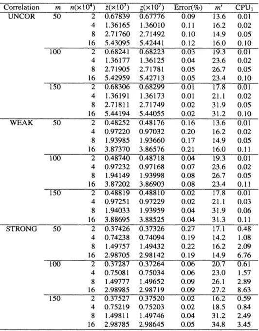
Table 2 gives the results ofcomputation of upper and lower bounds as well as the pegging testfor larger

instances with $n=20000\sim 160000$ and$m=50\sim 150$. The table shows the upper and lower bounds $(\overline{z}$ and

$\underline{z}$, respectively),and the column of $\grave$

Error$($%$)$’ gives their relative

errors

defined by 100 $\cdot(\overline{z}-\underline{z})’\underline{z}$. Applying thepegging test, some knapsacks are fixed either at$0$

or

1, and $m’$ shows the number of unfixed knapsacks,

i.e.,$m’$ $:=|M\backslash (K_{0}\cup K_{1})|$. $CPU_{1}$’ istheCPU time in seconds to computeupperand lowerbounds, aswell as

to

carry

out thepegging test. From this table, we observe thatthe pegging works effectively in reducing the

number of knapsacks. However,

we

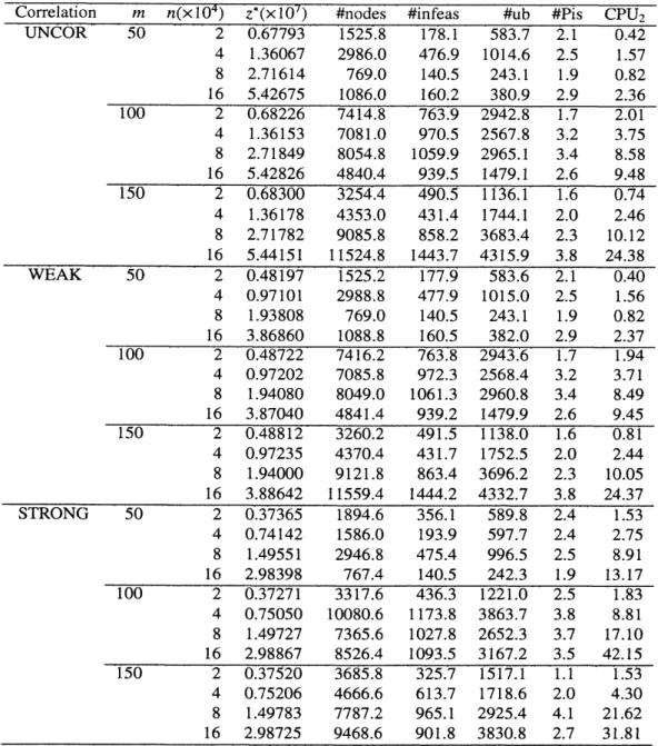
foundthatit isless effective for reducingthesize of$n$.

Table3 istheresults of the branch-and-boundalgorithm for various instances. This table showstheoptimal value $(z^{*})$, the number of the generated nodes in the branch-and-bound algorithm (#nodes), the number of

pruned subproblems dueto infeasibility(#infeas),

or

duetoupperbounds(#ub), the numberof terminalMKPs

solved by callingMULKNAP(#Pis), and theCPU time inseconds $(CPU_{2})$. Eachrowis againtheaverageover

10randominstances.

Except for

some

cases, thebranch-and-bound method solved BCMKPs exactly by invoking MULKNAP only

a

fewtimesand within

a

fewminutes. Weconclude that thebranch-and-bound algorithm isverysuccessful

for these largeinstances.

6 Conclusion

Wehaveformulatedthebudget-constrained multiple knapsack problem, and presented

an

algorithmto solve

this problem to optimality. By combining the Lagrangian relaxation and pegging test with the branch-and-boundmethod that solves MKPateachterminal nodesby callingMULKNAP,

we were

abletosolve almost all BCMKPs withupto $n=160000$items and$m=150$knapsacks within afew minutes in an$ordinai\gamma$computing

environment. However instances with smaller$n$and larger$m$remain hardtobe solved exactly.

References

[1] R.S. Dembo, P.L. Hammer, A reduction algorithm for knapsack problems, Methods ofOperations Re-search 36(1980)49-60.

[2] M. Fisher, The Lagrangian relaxation method for solving integerprogramming problems, Management

Science27(1981) 1-18.

[3] M.R. Garey, D.S. Johnson, Computers and Intractability: A Guide to the Theory of NP-Completeness, Freeman andCompany, SanFrancisco, 1979.

[4] ILOG, CPLEX11.1,http://www.ilog.com/products/cplex,2009.

[5] H. Kellerer,U. Pferschy,D. Pisinger, KnapsackProblems, Springer,Berlin,2004.

[6] S. Martello, P. Toth, Knapsack Problems: Algorithms and Computer Implementations, John Wiley&

Sons,Chichester, 1990.

[7] D. Pisinger, An expanding-core algorithm for theexact0-1 knapsack problem, European Joumal of Op-erational Research87 (1995) 175-187.

[8] D. Pisinger, An exact algorithm for large multiple knapsack problems, European Joumal ofOperational

Research 114 (1999)528-541.

[9] L. Wolsey, Integer Programming, John Wiley&Sons,NewYork, 1998.

[10] T. Yamada, T. Takeoka, An exact algorithm for the fixed-chargemultiple knapsack problem, European Joumal of Operational Research 192(2009) 700-705.

Table2: Bounding andpeggingresults for largeinstances.

$\overline{\frac{Corre1ationmn(\cross 10^{4})\overline{z}(\cross 10’)\underline{z}(\cross 10’)Error(\varphi_{0})m’CPU_{1}}{UNCOR5020.678390.677760.0913.60.01}}$

4

1.36165

1.36010 0.11 16.2 0.02 8

2.71760

2.71492 0.10 14.9 0.05 $\frac{165.430955.424410..1216.00..10}{10020.682410.6822300319.3001}$ 4 1.36177 1.36125

0.04

23.6 0.02 8 2.71905 2.71781 0.05 26.7 0.05

$\frac{0.05}{15020.683060.682990.0117.80.01}$

16 5.42959 5.42713 23.4 0.10 4

1.36191

1.36173

0.01

21.1

0.02

8 2.71811 2.71749 0.02 31.9 0.05 $\frac{165.441945.440550.0231.20.10}{WEAK5020.482520.481760.1613.60.01}$ 4 0.97220 0.97032 0.20 16.2 0.02 8 1.93985 1.93660 0.17 14.9 0.05 16

3.87370

3.86576 0.21 16.0 0.11 100 2

0.48740

0.48718

0.04

19.3 0.01 4 0.97232 0.97168 0.07 23.6 0.02 8 1.94149 1.93998 0.08 26.7 0.05 16 3.87202 3.86903 0.08 23.4 0.11 150

20.48819

0.48810 0.02 17.8 0.01 4 0.97251 0.97229 0.02 21.1 0.03 8

1.94033

1.93959

0.04

31.9

0.06

$\frac{163.886953.885250.0431.30.11}{STRONG5020.374260.373260.2717.10.48}$ 4 0.74238 0.74094 0.19 14.2 1.08 8 1.49757 1.49432 0.22 16.2 2.09 $\frac{162.987052.981420.19}{1(X)20.372870.372640.0620.70.61}$14.9 6.76 4 0.75081 0.75034 0.06 23.0 1.57 8 1.49777

1.49652

0.09 26.1 2.89 16 2.98985 2.98719 0.09 27.2 8.63 150 2 $0.375277$ _{037520 002 162 059} 4 0.75219 0.75203 0.02 18.5 0.84 8 1.49811 1.49746 0.04 31.2 2.49 16 2.98785 2.98645 0.05 34.8 3.45

Table3: Branch-and-boundresultsfor largeinstances.

Correlation $m$ $n(\cross 10^{4})$ $z^{*}(\cross 10^{7})$ $\#$ odes

#infeas

_仇市

#Pis

_{$CPU_{2}$}

$\overline{UNCOR502}$

0.677931525.8178.1583.72.10.42

4 1.36067 2986.0 476.9 1014.6 2.5 1.57 8 2.71614 769.0 140.5 243.1 1.9 0.82 $\frac{165.426751086.0160.2380.92.92.36}{10020.682267414.8763.92942.8172.01}$ 4 1.36153 7081.0 970.5 2567.8 3.2 3.75 8 2.71849 8054.8 1059.9 2965.1 3.4 8.58 $\frac{165.428264840.4939.51479.12.69.48}{15020.683003254.4490.51136.11.60.74}$ 4 1.36178 4353.0

431.4

1744.1 2.0 2.46 8 2.71782 9085.8 858.2 3683.4 2.3 10.12 $\frac{165.4415111524.81443.74315.93.824.38}{WEAK5020.481971525.2177.9583.62.10.40}$ 4 0.97101 2988.8 477.9 1015.0 2.5 1.56 8 1.93808 769.0 140.5 243.1 1.9 0.82 $\frac{163.868601088.8160.5382.02.92.37}{10020.487227416.2763.82943.6171.94}$ 4 0.97202 7085.8 972.3 2568.4 3.2 3.71 8 1.94080 8049.0 1061.3 2960.8 3.4 8.49 16 3.87040 $\frac{4841.4939.21479.92.\cdot 69.45}{15020.488123260.249151138.0160.81}$ 4 0.97235 4370.4 431.7 1752.5 2.0 2.44 8 1.94000 9121.8

863.4

3696.2

2.3 10.05 16 3.88642 11559.4 1444.2 4332.7 3.8 24.37 STRONG 50 20.37365 1894.6 356.1 589.8 2.4 1.53 4 0.74142 1586.0 193.9 597.7 2.4 2.75 8 1.49551 2946.8 475.4 996.5 2.5 8.91 $\frac{162.98398767.4140.5242.31..913.17}{10020.372713317.6436.312210251.83}$ 4 0.75050 10080.6 1173.8 3863.7 3.8 8.81 8 1.49727 7365.6 1027.8 2652.3 3.7 17.10 16 2.98867 8526.4 1093.5 3167.2 3.5 42.15 150 20.37520 36858 3257 15171 11 153 4 0.75206 4666.6 613.7 1718.6 2.0 4.30 8 1.49783 7787.2 965.1 2925.4 4.1 21.62 16 2.98725 9468.6 901.8 3830.8 2.7 31.81