Constrained Guided Spiral Transition Curves (Computer Algebra : Design of Algorithms, Implementations and Applications)

1

(14

Constrained Guided

Spiral

Transition Curves

Zulfiqar

Habib

*

and Manabu Sakai

\dagger

Kagoshima

University, Japan

$\mathrm{I}$

Abstract

A method for drawing a guided $G^{2}$ continuous cubic spiral spline curve that falls within a closed

boundary is presented. The boundary is composed of straight line segments and circular arcs. Spiral

segments consist oftransitionsfrom straight line to straight line or circle. Guidedcurve can easily be

controlledby shape controlparameter. Our scheme has better smoothness and moredegree of&aedom

thanany previous method. Alsoourscheme iscompletelylocal and hencemoresuitable andcomfortable

for practicaluse.

Keywords: cubic,guided,$G^{2}$spiral, constrained spline

1

Introduction

A method for drawing

a

guided $G^{2}$ continuous cubic spiral spline

curve

that falls within

a

closed boundaryis presented. Theboundaryis composed of straight line segments and circular

arcs.

Wediscuss cubic $G^{2}$ spiral transition from straight line to circle. Then

we

extend it for transition between two

non-parallel straight lines andfinally make it suitablefor constrained guided

curve.

Our constrained

curve

can easily be controlledby shapecontrol parameter. Any change in this shapecontrol parameter does not effect the continuity and neighborhoodparts of the

curve.

There

are

several problems whose

solutionrequiresthesetypesofmethods. Forexample

.

A

user

may wish todesigna

curve

thatfitsinsideagivenregion as,forexample, when

one

is designing

a

.

shapeto be cut from aflatsheetofmaterial.

A

user

may wishtodesign

a

smooth paththat avoids obstacles as, forexample, when

one

is designing

arobot

or

auto drive

car

path.

.

For applications such

as

the design of highways

or

railways it is desirable that

curve

be fair. In

the discussion about geometric design standards in AASHO (American Association of State Highway

Officials), Hickerson [6] (p. 17) states that “Sudden changes between

curves

ofwidely different radiior

between long tangents and sharp

curves

shouldbe avoided by the

use

of

curves

ofgradually increasing

or decreasing radii without at the

same

time introducing an appearance of forced alignment”. The

importance of this design feature is highlighted in [3] that links vehicle accidents to inconsistency in highwaygeometricdesign.

Parametric cubic

curves

arepopularinCADapplications because they

are

the lowest degree polynomial

curves

that allowinflection points (wherecurvature is zero), sothey

are

suitablefor the composition of $G^{2}$ splines. Tobe visually pleasing it isdesirablethat the spline befair. TheBezierformof

a

parametric cubic

curve

is usually usedin $\mathrm{C}\mathrm{A}\mathrm{D}/\mathrm{C}\mathrm{A}\mathrm{M}$ andCAGD (ComputerAidedGeometricDesign) applications

because of its geometric and numerical properties. Many authors have advocatedtheir

use

in different applicationslikedata fitting and fontdesigning. Theimportanceofusingfair

curves

inthe design process is well documented in the literature [2]. Cubic curves, althoughsmoother,

are

not always helpful since

theymight haveunwanted inflectionpointsand singularities(See[10]). Spirals haveseveral advantages of containingneitherinflectionpoints, singularities norcurvature extrema (See [5]). Such

curves are

useful

for transitionbetween two circles

or

straight lines.

$\mathrm{E}$mail: [email protected] Web: $\mathrm{h}\mathrm{t}\mathrm{t}\mathrm{p}://\mathrm{z}\mathrm{u}\mathrm{l}\mathrm{f}\mathrm{i}\mathrm{q}\mathrm{a}\mathrm{r}.8\mathrm{m}.\mathrm{c}\mathrm{o}\mathrm{m}$

$\uparrow \mathrm{E}$-mail:[email protected]–u.ac.jp, Department of Mathematics and Computer Science

tGraduateSchoolofScience and Engineering, Korimoto1-21-35, Kagoshima University, Kagoshima890-0065,Japan.

185

Many authors have discussed the problem of drawing constrained curves. In [4], a $G^{2}$ continuous,

shape-preserving curve made of rational cubics that interpolates to given points and that lies on one

side of

a

line, orseveral lines, is described. In [8], fair Bezier

curves

withfixed cross-sectional area are

produced. In [1], a $C^{1}$ continuous non-parametric interpolation rational (cubic numerator and linear denominator) that lies above, below, or between polylines is discussed. In [9],

a

$G^{2}$ continuous

curve

made of non-parametric rational cubics that lies ononesideofaline, or onesideofaquadratic curveis found.

Inour paper,the boundaryconsistsofstraight linesegmentsandcircular arcs, whichisdifferent than

boundariesconsidered by above mentionedpapers. Recently, Meek [7]presented amethodfor drawinga

guided$G^{1}$ continuous planar spline

curve

that falls within a closed boundarycomposedof straight line

segmentsand circles. $G^{1}$ continuity is not suitable for manypractical applications where high degreeof smoothness is required, for example, high way designing. Our guided

curve

has better smoothness than

Meek [7] scheme which has $G^{1}$ continuity. Theobjectives andshapefeaturesof

our

scheme inthispaper

are

.

Toobtain $G^{2}$ cubicspiral transition fromstraight line tocircle and make it moreflexible than Walton scheme in [11].

.

Toobtaincubic spiraltransitionbetweentwo non-parallelstraightlines.

.

To obtain guided $G^{2}$ continuous cubic spiral spline that falls within

a

closed boundary composed of

straight linesegmentsand circles.

.

To discuss and proveshapefeaturesof cubic spiral.

.

Toachieve

more

degreesoffreedom and flexibleconstraints for easy

use

inpractical applications.

.

Anychangeinshape parameterdoes not effectcontinuityandneighborhoodpartsof

our

guided spline.

So,our scheme is completely local.

Inthispaper, $\mathrm{x}$ standsforthetwodimensional

cross

product_{$(x_{0},y\mathrm{o})\mathrm{x}(x_{1},y_{1})=x_{0}y_{1}-x_{1}y_{0}$} and $||\cdot||$

means

the Euclidean norm. Let $L$be

a

straightline throughorigin$O$andacircle 0of radius$r$centered at $C$

.

Considerthe planarcurve$z(t)=(x(t),\mathrm{u}(\mathrm{t})$$0\leq t\leq 1$and for later use, consider

$\mathrm{u}(\mathrm{t})=u_{0}(1-t)^{2}+2u_{1}t(1-t)+u_{2}t^{2}$, $\mathrm{u}(\mathrm{t})=v_{0}(1-t)^{2}+2v_{1}t(1-t)+v_{2}t^{2}$ (1.1)

Aspiral isa

curve

whose curvature does notchangesignand whose curvatureis monotone. $G^{2}$ (Geometric continuity ofsecond order)

means

continuity in position, in unit tangent, and in signed curvature. A

curve is said to match $G^{2}$ Hermite data ifit passes from

one

given point to another given point, if its

unit tangentmatchesgiven unit tangentsatthe two given points, and its signed curvature matches given signed curvatures at the two given points.

This paperdoes not include discussion on PH quintic spiral due to page limitation, however it will

appear

soon

in

our

next paper. The organization ofour paper is as follows. We start from $G^{2}$ cubic

Bezier function, then description of methodfor spiral transition from straightlineto circle,its extension

for transition between nonparallel straight lines and finally application to constrained guided spline.

Numericalexamples, analysis, comparison and conclusions

are

given in last section.

2

Spiral

Transition

From Straight

Line to Circle

Weconsider

a

cubic transition$z(t)$ (seeFigure 1)of theform$\mathrm{z}’(\mathrm{t})=(u(t),v(t))$

.

Itssignedcurvature

$\kappa o)$ isgiven by

$\kappa(t)(=’\frac{z(t)\mathrm{x}z(\prime t)}{||z\zeta t)||^{s}},’)=\frac{u(t)v’(t)-u’(t)v(t)}{\{u(t)^{2}+v^{2}(t)\}^{3/2}}$ (1.1)

Forlateruse, consider

$\{u^{2}(t)+v^{2}(t)\}^{5/2}\mathrm{z}’(\mathrm{t})=$ $\{u(t)v’’(t)- u"(t)\mathrm{z}\mathrm{r}(t)\}$$\{u^{2}(t)+v^{2}(t)\}$ (2.2)

-3$\{u(t)v’(t)-u’(t)v(t)\}\{u(t)u’(t)+v(t)v’(t)\}(=$u(t)

Here, werequirefor $0<\theta<\pi/2$

166

Figure 1: Cubicspiral transition from straight line to circle.

Then, the above conditionsrequire

Lemma 2.1. With apositive parameter$d$

$u_{1}= \frac{d^{2}}{2r\sin\theta}$, _{$u_{2}=d\cos\theta$}, _{$v_{0}=0,$ $v_{1}=0,$ $v_{2}=d\sin\theta$} (2.4)

where$\mathrm{z}’(0)=(\mathrm{u}\mathrm{o}, 0)$ and$\mathrm{z}’(0)$ $=d(\cos\theta,\sin\theta)$

.

We introducea pairofparameters $(m,q)$for $(\mathrm{u}\mathrm{o}, d)$

as

$u_{0}=mui,$$d=qr$, Then

$u_{0}= \frac{mrq^{2}}{2\sin\theta}$, $u_{1}= \frac{rq^{2}}{2\sin\theta}$,

$u_{2}=qr\cos\theta$, $v_{0}=v_{1}=0,$ $v_{2}=qr\sin\theta$

from which

(2.5)

from which

$x(t)= \frac{qrt}{6\sin\theta}[q\{(3-2t)t+m(3-3t+t^{2})\}+t^{2}\sin 2\theta]$ _, $y(t)= \frac{qrt^{\delta}\sin\theta}{3}$ (2.5)

Walton ([11]) consideredacubic

curve

$z(t)$($=$ v(t))$y(t)))$,$0\leq t\leq 1$ofthe form

$z(t)=$bo$(1-t)^{3}+3b_{1}t(1-t)^{2}+362(1-t)t^{2}+b_{3}t^{3}$

where B\’ezierpoints $b_{\dot{l}}$,$0\leq i\leq 3$

are

defined

as

follows

(2.7)

where B\’ezierpoints $b_{\dot{l}}$,$0\leq i\leq 3$

are

defined

as

follows

$b_{1}-b_{0}=b_{2}-b_{1}= \frac{25r\tan\theta}{54\cos\theta}(1,0)$, $b_{3}-b_{2}= \frac{5r\tan\theta}{9}(\cos\theta,\sin\theta)$ (2.8)

Simplecalculation gives

$x’(t)$($=$v(t)) $=$vo$(\mathrm{l}-t)^{2}1$ $2u_{1}t(1-t)+u_{2}t^{2}$, $y’(t)(=v(t))=$vo$(\mathrm{l}-t)^{2}+2v_{1}t(1-t)+v_{2}t^{2}$ (2.9)

where

$u_{0}=u_{1}= \frac{25r\tan\theta}{18\cos\theta}$, $u_{2}= \frac{5r\sin\theta}{3}$, _{$v_{0}=v_{1}=0,$} $v_{2}= \frac{5r\tan\theta\sin\theta}{3}$ (2.4)

Hence, notethat theirmethod isour specialcasewith $m=1$ and $q= \frac{5}{3}\tan\theta$.

With help ofa symbolic manipulator, weobtain

$\kappa$

’(

$\frac{1}{1+s})=\frac{8(1+s)^{6}(\sum_{=0}^{5}a_{i}s^{i})\sin^{3}\theta}{r\{q^{2}s^{2}(2+ms)^{2}+2qs(2+ms)\sin 2\theta+4\sin^{2}\theta\}^{5/2}}.\cdot$

(2.4)

where

$a_{0}=4\{3q\mathrm{c}o\mathrm{s}\theta-(4+m)\sin\theta\}\sin$J9, _{$a_{1}=2\{6q-2q(5-4m)\sin 2\theta-10m \sin 2 \theta\}$}

$a_{2}=2q$

{

$(-2+$13m)g$-2m(4-m)\sin 2\theta$

}

, _a3 $=2mq$

{

$(-3+$10m)g$-2m\sin 2\theta$

}

$a_{4}=5m^{3}q^{2}$, $a_{6}=n^{3}q^{2}$

Hence, wehavea sufficient spiralconditionforatransition curve$\mathrm{z}(t)$,$0\leq t\leq 1,$i.e.,$a_{\mathrm{i}}\geq 0,0\leq i\leq 5$

167

Lemma 2.2. The cubic segment$z(t)$,$0\leq t\leq 1$

of

the

form

(1.1) is aspiral satisfying (2.4)

if

$m>3/10$

and

$q\geq q(m, \theta)(={\rm Max}\{$$\frac{(4+m)\tan\theta}{3}$, $\frac{2m(4-m)\sin 2\theta}{13m-2}$, $\frac{2m\sin 2\theta}{10m-3}$,

$\frac{1}{6}\{(5-4m)\cos\theta+$ cosO$+(5-4\mathrm{r}\mathrm{n})^{2}$

cos2

$\theta\}\sin$$\theta])$ (2.12)

Theorem 2.1. The cubic segment $z(t),0<t\leq 1$

_of

the

_for

$rm(\mathit{1}.\mathit{1})$ is a spiral satisfying (1.1) and

$\kappa’(1)=0$

for

$\theta\in(0, \pi/2]$

if

$m\geq$ 2(-l $+\sqrt{6}$)$\overline{/}5(=c_{0})(\approx$ 0.5797$)$

Proof.

Letting$z$$=\tan\theta(>0)$, we only have tonotethat thetermsinbrackets of(2.11) reduce

$\frac{(4+m)z}{3}(=A_{1})$,$\frac{4m(4-m)z}{(13m-2)(1+z^{2})}(=A_{2})$,$\frac{4mz}{(10m-3)(1+z^{2})}(=A_{3})$, $\frac{z\{5-4m+\sqrt{25+16m^{2}+20m(1+3z^{2})}\}}{6(1+z^{2})}(=A_{4})$

Here, wehave tocheck that the firstquantity is not less than the remainingthreeones where

$A_{1}\geq A_{2}$ $(m \geq\frac{1}{25}(-1+\sqrt{201})(\approx 0.5270))$

$A_{1}\geq A_{3}$ $(m \geq\frac{1}{20}(-25+\sqrt{1105})(\mathrm{z} 0.4120))$, $A_{1}\geq A_{4}$ $(m\geq c_{0})$

口

3

Family of

Spiral

Transitions

Between Two Straight

Lines

Figure2: Cubic spiraltransitionbetweentwo straight lines.

Here,wehave extended the idea of straight line to circle transition andderived

a

method forBezier

spiraltransitionbetween two nonparallel straight lines (seeFigure 2). We note the followingresult that isof

use

for joining two lines. For$0<\theta<$ $\mathrm{r}/2$, weconsider

a

cubiccurvesatisfying

$\mathrm{z}(0)=(0,0)$, $z’(0)||(1.1)$, $\kappa(0)=$ l/r, $z’(1)||(\cos\theta,\sin\theta)$, $\kappa(1)=0$ (3.1)

Since B\’ezier

_{curves are}

affine invariant,

a

cubic B\’ezier spiral can be used in

a

coordinate free

man-ner. Thereforetransformation, i.e., rotation, translation, reflectionwith respect to$y$-axis andchange of variable$t$with $1-t$to (2.6)gives $z(t)(=\mathrm{x}(\mathrm{t})\mathrm{y}(\mathrm{t})$by

$\mathrm{x}(\mathrm{t})=\frac{qrt}{6\sin\theta}[qt\{3-(2-m)t\}\cos\theta+2(3-3t+t^{2})\sin\theta]$

188

Now,$\mathrm{z}(\mathrm{t},\mathrm{m},\mathrm{O})(- (x(t,m,\theta),y(t,m, \theta))),0\leq t\leq 1$ denotes the cubicsplinesatisfying (3.1). Assumethat

the anglebetween two lines is7 $(<\pi)$

.

Then, $(x(t,m,\theta_{0}),y(t,m,\theta_{0}))$ of the form (3.2) with $q=q_{0}(\geq$

$\mathrm{q}\{\mathrm{m}$,Qo)) and $(-x(t,n,\theta_{1}),y(t, n,\theta_{1}))$of the form (3.2) with $q_{1}$($\geq$ q{m,Qo)$)$ with$\theta_{0}+\theta_{1}=\pi$_$-\gamma$is

a

pair

ofspiral transition

curves.

Figures $3(\mathrm{a}, \mathrm{b})$ shows the graphs of the family of$G^{2}$ cubic spiral transition

curves

between two straight linesfor $(\gamma,\theta_{0},\theta_{1})=(5\pi/12, \pi/4,\pi/3)$, (a) $(m_{0},m_{1})=(3,0.8)$ (shaded) and

$(1, 1)$ _{(bold), (b)} $r=0.1$ (shaded) and 0.2 (bold). Here start and end points of straight lines arenot fixedanduser has

no

control

over

them. This situation is not suitable for

some

practical applications.

3.1

Scheme

For Fixed

End

Points

When $\theta_{0}=\theta_{1}$ ($=\theta=(\pi-$y)/2)

are

fixed and $m,n\geq$ Cg (then, note $q_{0}=(4+m)/3\tan\theta$ and

$q_{1}=(4+n)/3\tan\theta)$, the distances between the intersection $O$ of the two lines and the end points

$P_{i},i=0,1$ofthe transition

curves

aregiven by $d(m,n,r,\theta)$ and $d(n,m,r, \theta)$ where

$\mathrm{d}\{\mathrm{m},\mathrm{n},\mathrm{r},\mathrm{O}$) $=(r/c)$$\{4+(3+m)^{3}+3(3+n)\}$

,

$c$$=54$

cos2

$\theta/\sin\theta$ (3.3)

Here

we

derive

a

condition

on

$r$for whichthe followingsystem ofequations hasthe solutions$m$,$n$($\geq$ q)

for given nonnegative$d_{0},d_{1}$

$d(m,n, r,\theta)=d_{0}$, $\mathrm{d}\{\mathrm{m},\mathrm{n},\mathrm{r},0$) $=d_{1}$ (3.4)

Let (a ) $=(3+m,3+n)$ reduce the abovesystemto

$\alpha^{3}+3\beta$$=\lambda$(_$=$ch/r-4), $\beta^{3}+3\alpha=\mu(=cd_{1}/r-4)$ (3.5)

where require $m,n\geq c_{0}$ to note$\mathrm{a},\#\geq c_{1}$$(=c_{0}+3)$ and $\lambda$,_{$\mu\geq c_{2}$}($=c_{1}^{3}+$3ci). Delete$\alpha$ from (1.23) to

get aquarticequation $\mathrm{f}(/3)=0$

$f(\beta)=\beta^{9}$-$3\mu\beta^{6}+3\mu^{2}\beta^{\theta}-81\beta+27\lambda-\mu^{3}$ (3.6)

Restrictions: $\alpha,$$\beta\geq c_{1}$ requirethat at least

one

root $\beta$of$f(\beta)=0$must satisfy

$c_{1}\leq\beta\leq(\mu-3c_{1})^{1/3}$ (3.7)

Intermediate valueof theoremgives

a

sufficientcondition: $f(c_{1})\leq 0$and$f((\mu-3c_{1})^{1/3})2$ $0$ where

$f(c_{1})=-7^{\mathrm{i}}’+$$3c7\mu^{2}-3c\mathrm{j}\mu$ $+$$27\lambda$_{$+$ $c_{1}^{9}-81c_{1}$ $=-$}$\{\mu-c\mathit{1}$ $-3(\lambda-3\mathrm{C}1)1/3\}$ $\mathrm{x}$

$[(\mu-c_{2})^{2}+3$$\{2c_{1}+$$(\lambda-3c_{1})^{1/}\mathrm{i}$$(\mu-c_{2})+9\{c_{1}^{2}+$Cl$(\lambda-3c_{1})^{1/3}+$$(\lambda-3\mathrm{C}1)1/3\}$

(3.8)

$f((\mu-3c_{1})^{1/3})=27\{\lambda-c_{1}^{3}-3(\mu-3c_{1})^{1/3}\}$

Sincethe quantity in bracketsis positivefor $\mu\geq c_{2}$, the sufficient

one

reduces to

$\lambda-c_{1}^{3}\geq 3(\mu-3c_{1})^{1/3}$, $\mu-c_{1}^{3}\geq 3(\lambda-3c_{1})^{1/3}$ (3.9)

Note$\lambda,\mu 2$$c_{2}$ to obtain

Lemma3.1. Given$h$,$d_{1}$,

assume

that$r$

satisfies

$\lambda-c_{1}^{3}\geq 3(\mu-3c_{1})^{1/3}\geq 0,\mu-$$\mathrm{c}’\geq 3(\lambda- 3\mathrm{c}_{1})^{1/3}$ $\geq 0.$

Then the system

_of

(3.5) has the reqgeiredsolutions $\alpha,\beta(\geq c_{1})$

.

Note $\lambda,\mu=$ O(l/r),$\mathrm{r}arrow \mathrm{t}$$0$ toobtain that asmall value of$r$ makestheinequalities (3.9) be valid for

any $h$,$d_{1}$

.

Next, for

an

upperbound for $r$,werequire

Lemma3.2.

_If

₄₂

$d_{1}$, then$\mu-c_{1}^{l}=3(\lambda-3c_{1})^{1/3}$ and$\lambda$,_{$\mu\geq c_{2}$} by (S. 5) hasauniquepositive solution

$r^{*}$

.

Restrictions: $\alpha$,$\beta\geq c_{1}$ requirethat at least

one

root $\beta$of$f(\beta)=0$must satisfy

$c_{1}\leq\beta\leq(\mu-3c_{1})^{1/3}$ (3.7)

Intemediatevalueof theoremgives

a

sufficientcondition: $f(c_{1})\leq 0$and$f((\mu-3c_{1})^{1/\theta})\geq 0$ where $f(c_{1})=-\mu^{3}+3c_{1}^{\theta}\mu^{2}-3c_{1}^{6}\mu+27\lambda+c_{1}^{9}-81c_{1}=-\{\mu-c_{1}^{3}-3(\lambda-3c_{1})^{1/3}\}\mathrm{x}$

$[(\mu-c_{2})^{2}+3\{2c_{1}+(\lambda-3c_{1})^{1/3}\}(\mu-c_{2})+9\{c_{1}^{2}+c_{1}(\lambda-3c_{1})^{1/3}+(\lambda-3c_{1})^{2/3}\}]$

(3.8)

$f((\mu-3c_{1})^{1/3})=27\{\lambda-c_{1}^{3}-3(\mu-3c_{1})^{1/3}\}$

Sincethe quantity in bracketsis positivefor $\mu\geq c_{2}$, the sufficient

one

reduces to

$\lambda-c_{1}^{3}\geq 3(\mu-3c_{1})^{1/3}$, $\mu-c_{1}^{S}\geq 3(\lambda-3c_{1})^{1/3}$ (3.9)

Note$\lambda,\mu\geq c_{2}$ to obtain

Lemma3.1. Given$h$,$d_{1}$,

assume

that$r$

satisfies

$\lambda-c_{1}^{3}\geq 3(\mu-3c_{1})^{1/3}\geq 0,\mu-c_{1}^{3}\geq 3(\lambda-3c_{1})^{1/3}\geq 0.$

Then the system

_of

(3.5) has the $[] rquired$solutions $\alpha,\beta(\geq c_{1})$

.

Note $\lambda$,

$\mu=O(1/r)$,$rarrow 0$toobtain that asmallvalueof$r$ makestheinequalities (3.9) be valid for

any $h$,$d_{1}$

.

Next, for

an

upperbound for $r$,werequire

Lemma3.2.

_If

$h$ $\geq d_{1}$, then$\mu-c_{1}^{l}=3(\lambda-3c_{1})^{1/3}$ and$\lambda,\mu\geq c_{2}$ by (3.5) hasauniquepositive solution

1

$6\theta$

Proof.

Let $t=$ 1/r toreduce$\mu-c_{1}^{3}=3(\lambda-3c_{1})^{1/3}$ to

$f(t)$ $(=(edit-4-c_{1}^{3})^{3}-27(\mathrm{c}\mathrm{d}\mathrm{o}\mathrm{t}-4-3c_{1}))=0$

where $\lambda,\mu 2$ $c_{2}$ are equivalent to$t\geq(c_{2}+4)[(cd_{1})$

.

First, note with $4=k^{2}d_{1}(k\geq 1)$

$f(+\infty)=+\infty$, $f( \frac{c_{2}+4}{cd_{1}})=-27(c_{1}+1)(c_{1}^{2}-c_{1}+4)(k^{2}-1)(\leq 0)$

In addition, $f(t)$ has its relative maximum at $t=$ ($c_{1}^{3}+4-$ Sk)/(cdi)$(< (c_{2}+ 4)/(cd_{1}))$

.

Therefore,

$\mathrm{f}(\mathrm{t})=0$ has just

one

root $t=t^{*}(=1/r^{*})$($\geq(c_{2}+$4)/(cdi)). $\square$口

As $r$ increasesfrom zero, “equality” in the second inequality of(3.9) isfirstvalid. Hence,

we

obtain

Theorem 3.1. Assume that$d_{0}\geq d_{1}$

.

Then the system

of

equation (3.4) in $m,n$ ($\geq$ Co) is solvable

for

$0<r\leq r^{*}$ where$r^{*}$ is the positive rootno greater than_{$cd_{1}/(c_{2}+4)$}

$\{(4+c_{1}^{3})r-cd_{1}\}^{3}-27r^{2}$$\{(4+ 3\mathrm{c}\mathrm{i})) -d_{0}\}$ _$=0,$ $c_{1}=\mathrm{c}_{0}^{3}+3c_{0}$ (3.11) Then,

_for

the angle $\gamma(<\pi)$ between the two straight lines with $0=(\pi- 7)$/2, ($x$(t,$m,\theta$), $y(t,m,\theta)$),

$q=\{(4+m)/3\}$$\tan\theta$

of

the

form

(S. 2) and $(\mathrm{x}(\mathrm{t},\mathrm{m},9), \mathrm{y}(\mathrm{t},\mathrm{m}\mathrm{y}9))$, $q=\{(4+n)/3\}\tan\theta$

of

the

form

(3.2) is apair

_of

spiral transition

curves

between the two lines.

(a)Given$r=0.2$ (b) Given$(m,n)=$$(1, 1)$ (c) Given (do,$d_{1}$) $=(1,3)$

Figure3: Graphs of$z(t)$ with non-fixed $(\mathrm{a}, \mathrm{b})$ and fixed (c) start andend points.

Thisresult enables the pairofthe spirals topassthroughthegiven pointsof contactonthe nonparallel two straight lines. For example, in Figure $3(\mathrm{c})$, straight lines are given with $7=\theta_{0}=\theta_{1}=\pi/3$,

$r=0.1$ (shaded) and 0.2 (bold). By (3.4), for $r=0.1$, $(\mathrm{m}\mathrm{o},\mathrm{m}\mathrm{i})\approx(4.65,2.05)$ and for $r=0.2,$

$(\mathrm{m}\mathrm{o}, m_{1})\approx(3.02,0.82)$

.

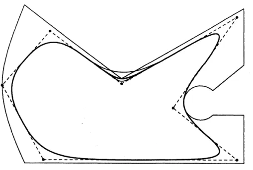
To keep the transition curvewithin a closed boundary, value of shape control

parameter $r$ can be derived from (3.2) when control points and boundary information are given. A

constrainedguided

curve

isshown in Figure 4.

4

Examples,

Analysis

and

Conclusion

In Figure4,

a

constrained$G^{2}$ continuous cubic spiralspline

uses

straightline tostraightlinetransition. Theboundaryis composedof straight line segments and circular

arcs.

These

curves

areguidedby shape control parameter and all segments have completely local control, i.e., any change in

one

segment does not effectcontinuityand shapeof neighboringsegments. The data for boundary and controlpoints has been takenfrom Figure 8in [7] whichhas $G^{1}$ continuity and scheme is notcompletely local.

Cubicspiral segments

are

usefulin the design of objects when it is desirablethatfair

curves

be used

in the designprocess. A method forstraight line to circletransition has beendiscussed and extendedto

transition

curve

between two

non

parallel straight lines. We proved that Walton scheme for cubic [11]

isa special

case

of

our

most flexible scheme. We offered reasonable degreeof freedom and extendedour

schemes to $G^{2}$ guided spiral spline constrained by a closed boundary. Our scheme has $G^{2}$ continuity which is better than $G^{1}$ continuity in [7]. $G^{1}$ continuity is not suitable for many practical applications where high degree ofsmoothness is required.

170

Figure4: A $G^{2}$ cubicguided spiral spline constrained by aclosed boundary.

References

[1] Q. Duan, G. Xu, A. Liu, X. Wang, and F. Cheng. Constrained interpolationusing rational cubic

spline

curves

with linear denominators. Korean Journal

_of

Computational

8

Applied Mathematics, 6:203-215, 1997.

[2] G. Farin. Curves and

_{Surfaces for}

Computer Aided GeometricDesign: A Practical Guide. Academic

Press, NewYork, 4th edition, 1997.

[3] G. M. Gibreel, S. M. Easa,Y. Hassan, and I. A. El-Dimeery. State ofthe art of highway geometric

design consistency. ASCE Journal

_of

$\mathfrak{W}nspo\hslash ation$Engineering, 125(4):305-313,1997.

[4] B. H. Goodman, T. N. T. Ong and K. Unsworth. NURBS

for

Curve and

_Surface

Design., chapter ConstrainedInterpolation Using Rational Cubic Splines, pages59-74. SLAM, Philadelphia, 1991.

[5] Z. Habib and M. Sakai. $G^{2}$ planar spiral cubic interpolation to a spiral. pages 51-56, USA, July

2002. The Proceedings ofIEEE International Conference

on

Information Visualization-IV’02-UK, IEEEComputer Society Press.

[6] T. F. Hickerson. Route Location and Design. McGraw-Hill, NewYork, 1964.

[7] D. S. Meek, B. Ong,and D. J. Walton. A constrained guided$G^{1}$ continuous spline

curve.

Computer Aided Design, 35:591-599,2003.

[8] H. Nowacki and X. Lu. FairingB\"ezier

curves

with constraints. Computer Aided Geometric Design, 7:43-55, 1990.

[9] B. Ong. Mathematical Methods in Computer Aided Geometric Design, chapterOn Non-parametric

ConstrainedInterpolation, pages 419-430. Academic Press,Philadelphia, 1992.

[10] M. Sakai. Osculatory interpolation. Computer Aided Geometric Design, 18:739-750,2001.

[11] D. J. Waltonand D.S.Meek. A planar cubic Bezier spiral. Computationaland Applied Mathematics,