Progressive Application of a Lagrangian Vortex Method into Fluid Engineering and Possibility of the Concept of Discrete Element Methods in Vortex Dynamics (Mathematical analysis of the Euler equations : 150 years of vortex dynamics)

Progressive Application of

a

Lagrangian Vortex Method into

Fluid

Engineering

and Possibility

of

the Concept of

Discrete

Element

Methods in

Vortex

Dynamics

Kyoji Kamemoto ProfessorEmeritus, DepartmentofMechanical Engineering, YokohamaNational University 1. Introduction

The vortex methods have been developed and applied for analysis ofcomplex, unsteady

and vortical flows in relation to problems in awide range ofindustries, because they consist

ofsimple algorithm based

on

physics offlow. Nowadays, applicability ofthe vortex element

methods has been developed and improved dramatically, and it has become encouragingly clear that the vortex methods have

so

much

interesting

features thatthey provide researchers and engineers with easy-to-handle and completely grid-ffee Lagrangian calculation of

unsteady and vortical flows without

use

of any RANS type turbulence models.

Leonardl

summarized the basic algorithm and examples of its applications.

Sacpkaya2

presented a comprehensive review ofvarious vortex methods based

on

Lagrangian ormixed Lagrangian-Eulerian schemes,theBiot-Savart law

or

the vortex incell methods.

Kamemoto3

summarized the _{mathematical basis}oftheBiot-Savartlawmethods. Recently,

Kamemoto4

reportedseveral attractive applications involving simulation of various kinds of unsteady flows with

an

advanced vortex method, and Ojima and

Kamemoto5

reported interestingresultsof

a

studyon

numerical simulation of unsteadyflows arounda swimming fishbyusing theirvortexmethod.

As well

as

many finite difference methods, it is

a

crucial point in vortex methods that the number of vortex elements should be increased when higher resolution of turbulence

srucmres

is required, and then the computational time increases rapidly. In order to reduce

the operation count of evaluating the velocity at each vortex element

or

particle $throu\phi$

a

Biot-Savart law, fast$N$-body solvers, by which the operation count is reduced Rom _$O(N)$ to

$O(N\log N)$, have been proposed by Greengard and

Rohklin.6

On the other hand, in order to

reduce the computational load incalculation of mrbulence stmcmres, Fukuda and

Kamemoto7

proposed

an

effective redistribution model of vortex elements with consideration of

convective motionandviscous diffisionin

a

three-dimensionalcore-spreading model.

Recently, in orderto expandthe applicability of the advanced vortex method,the group of

the presentauthor has made attempts to applyit into fiirther complicatedand vorticalflows in

several fields. Kamemoto and

Ojima8

applied the method into the fluid dynamics in sports

science, and they simulated three-dimensional, complex and unsteady flows around

an

isolated 100 $m$

runner

and also aski-jumper. Iso and

Kamemoto9

developed a coupled vortex

method and particle method analysis tool for numerical simulation of intemal unsteady two-phase flows, and they numerically simulated intemal liquid-solid two-phase flows

in

a

vertical channel and

a

mixing tee. Furthemiore, expanding the concept of the Lagrangian vortex methodin whichvorticitylayers

are

expressed byanumber ofdiscrete vortexelements,

Ishimoto$1$

and the group of the present author have attempted numerical simulation of behavior ofplasmain

a

magnetic fieldbyintroducing superparticles of electrons.

In tins paper, in order to overview the recent attempts, the mathematical background

and numerical procedure of the advanced vortex method applied to the recent studies

are

briefly explained andthe progressive studies

on

simulation of such hard-to-solve and vortical flows

as

the complex flows around a 100 $m$ runner, the liquid-particle two phase flows in a

channel and the vortical motionof plasma cloudsin

a

magnetic field

are

digested. And finally,

a

new direction of ffinher development of the vortex element dynamics is viewed in conclusion.

2.Algorithms of Lagrangian Vortex Element Method

The govening equations for viscous and incompressible flow

are

described with the vorticitytransportequation and thepressurePoisson equation, which

can

be derivedbytaking the rotationand the divergence ofNavier-Stokes equations, respectively.

$\frac{\partial w}{\partial t}+(u\cdot\Psi^{ad)w}=(\Phi\cdot\Psi^{ad)u+\Pi^{2}q)}$ (1)

$\forall p=\rho div$($u$

.

grad

u) (2)

Where $u$ is

a

velocity vector, and $v$ and $\rho$ respectively denote kinematic viscosity and fluid

density. The vorticity $\omega$ is defined

as

$a=rotu$. As explained by Wu and Thompson$1^{}$ , the

Biot-Savart law

can

bederived ffom the definition equationofvorticity

as

follows.

$u= \int_{V}(\omega_{0}x\nabla_{0}G)dv+\int_{s}\{(n_{0}\cdot u_{0})\cdot\nabla_{\theta}G-(n_{0}xu_{0})x\nabla_{0}G\}ds$ (3)

Here, subscript $0$

” in

Eq.(3) denotes variable, differentiation and integration at

a

location $r_{0}$,

and $n_{0}$ denotes the normal unit vector at

a

point

on

a

boundary surface $S$. And $G$ is the

fundamental solution ofthe scalar Laplace equation with the delta hmction 6$(r- r_{0})$ intheright

hand side, which is written

as

$G=1/(4\pi|r- r_{o}|)$ for

a

three-dimensional field. In Eq. (3), the

inner product $(n_{0}. u_{0})$ and the outer product $(n_{0}\cross u_{0})$ stand for respectively normal and tangential velocity components

on

the boundary surface, and they respectively correspond to

source

and vortex distributions

on

the surface. Therefore,

_as

shown in Fig.1, it is mathematically understood that avelocity field ofviscous and incompressible flowis amived

at the field integration conceming vorticity distributions in the flow field and the surface integration conceming

source

andvortexdistributions around the boundary surface.

Instead ofthe finite difference calculation ofthe

pressure

Poisson equation representedby Eq. (2), the

pressure

in the flow field is calculated ffom the

integration

equation, which

was

formulatedby

Uhlman12

as

follows.

$\beta H+\int_{s}H\frac{\partial G}{\partial n}ds=-\int_{V}\nabla G(ux\omega)d\nu-\int_{s}\{G\cdot n\cdot\frac{\partial u}{\partial t}+\nu\cdot n\cdot(\nabla Gx\omega)\}ds$ (4)

Here,$\beta$ is _$\beta=1$ inside the flow and _$\beta=1/2$

on

the boundary S. _$H$is the Bemoulli function

defined

as

$H=P/\rho+|u|^{2}/2$. _{The valueof}$H$

on

the boundary surface is calculated ffom Eq. (4)

byusingthe panelmethod.

One of the most important schemes in the vortex method is how to represent the distribution of vorticity in the proximity of the body surface, taking account of viscous di$\mathfrak{N}sion$ and convection of vorticity under the non-slip condition

on

the surface. In the

present method,

a

thinvorticitylayer isconsidered along the solidsurface, _{and discrete}vortex

elements

are

introduced into the surrounding flow field considering the diffision and convection ofvorticityffomdiscrete elements ofthe$t!\dot{u}n$ vorticitylayerwith vorticity $\omega$

.

The

details of treatnents have been explained in the paper written by Ojima&Kamemoto

13.

It will be noteworthy that

as a

linear distribution of velocity is assumed in the thin vorticity layer, the ffictional stress

on

the wall surface is evaluated approximately Rom the following equation

as

$\tau_{w}=\phi u/\partial n=-\mu\omega$

.

Once the pressure distribution and frictional stress around

the boundary surface

are

calculated, integration of the pressure and the shearing stress along

the surface yields the force acting on the body. When a vortex element, which is introduced

into the surroundingfield, _{flows downstream and far ffom the solid} surface,it

can

bereplaced

with

an

equivalent discrete vortex element for simplification of numerical treatment by

considering conservation of vortex strength. The discrete vortex element is modeled by

a

vortex blob which has

a

spherical structure with

a

radial symmetric vorticity distribution

proposed by Winkelmans

&Leonardl4.

The motion of the discrete vortex elements is

representedby Lagrangianfomi of

a

simpledifferential equation$dr/dt=u$

.

_{Then,trajectory of}

a

discrete vortex element

over

a

time step is approximately computed Rom the Adams-Bashforth method. On the otherhand, the evolution ofvorticity is calculated by Eq.(l) with the three-dimensional

core

spreading method proposed by Nakanishi

&Kamemotol5.

It should be noted here that in order to keep higher accuracy in expression of

a

local vorticity

distribution, a couple ofadditional schemes ofre-distribution of vortex blobs

are

introduced

in thepresentadvanced vortexmethod. Whenthe vortex core of

a

blob becomes larger than a

representative scale of the local flow passage, the vortex blob is divided into

a

couple of

smallerblobs. On the otherhand, ifthe rate ofthree-dimensional elongation becomes largeto

some

extent, the vortex blob is discretized into plural blobs in order to approximate the

elongated vorticity distribution much

more

properly. The detail ofthe redistribution model is explainedinthe

paper

writtenbyFukuda and

Kamemoto7.

3. Progressive Applications

3.1Application to sports aerodynamics

In the study of numerical simulation of the flows around a 100 $m$

runner

and a

ski-jumper by Kamemoto and

Ojima8,

anumerical model ofa moving athlete is represented by distributing 3,020 quadrilateral panels around its body-sutface

as

shown in Fig.2 (a). For the moving conditions of each panel, the

new

co-ordinates ofeachpanel, instantaneous velocity and acceleration ofthe panel movement

are

given at each time step, and the

one

cycle of motion is produced by $320steps$ ofinstantaneous body configuration

as

shownin Fig.2 (b) in

which only eight characteristic steps of instantaneous running style are shown. The moving boundary data

are

imported into the calculation at each time step, which

are

used to change

both the configuration of athlete body and the boundary condition during the calculation of the flow field around the moving body. In order to examine the influence of runner’s posture,

calculations offlows around

a runner

with different forward-bent angles $(a=0^{o},$ $10^{o}$

.

$20^{o}$

.

$30$

$0)$ shown in Fig.2 (c)

were

perfomied. Moreover,

a

much

more

realistic flow around the

nmner was

simulated by introducing continuous variationof the forward-bent angle ffom 5$0^{0}$

to $0^{o}$ degree withthe elapsed time.

(a)Paneldistribution (b)One cycle of runningmotionat$a=0^{o}$ (c)Definition of forward-bentangle$a$

Fig.2 Representation ofabody configuration by quadrilateral panels.

In the study, in orderto normalize length scale,the breadth ofthe runner’s shoulders 0.4$m$

was

used

as

the representative length $L$ for normalization of the length scale. The assumed

mmuing speed 10 $m/s$

was

used

as

the representative velocity $U$ for normalization of the

velocity scale. As

one

cycle motion

was

represented 320 steps of instantaneous body configuration, and

as

it is known that

one

cycle of sprint rumuing motion of

a

first class

runner

takes approximately 0.45 $s$, the size of time step of the present time marching

calculations

was

taken to be $1.40x10^{-3}s$

.

_{The kinematic viscosity} $\nu$ and density $\rho$ of the

atmosphere

were

respectively assumed

as

$1.43\cross 10^{5}m^{2}/s$ and 1.2 $kym^{3}$

.

Therefore, the

Reynolds number of the flowaround the

runner

becomes $Re=UL/v=2.8$xl$0^{5}$

.

Figure 3 shows four views ofinstantaneous pressure distributions around the runner’s body

surface atthe bent angle $a=0^{o}$

.

Itis clearly observed that higher pressure regions

are

formed

onthe face and ffontal surfaces of body and the leftleg, and lowerpressure spots are formed

on the back and side surfaces of body and the

rear

surface ofthe left foot. And it has been

(a) $t=1.8\sec(a=30^{o})$

about 18 $N$ which corresponds to the value of drag coefficient Cd $\sim 0.8$

on

the assumptionof

dragarea as about 0.4$m^{2}$.

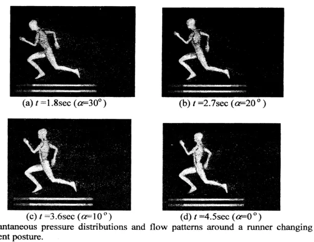
Figure 4 shows instantaneous pressuredistributions and flow pattems around

a

runner

who

is continuously changing forward-bentposture from 5$0^{0}$ to $0^{o}$. It is

seen

inthis figure that the

width of the wake formed behind therunneratthe forward-bent angle is 3$0^{0}$ is

narrower

and

it becomes wider asthe forward-bent angle becomes smaller. It hasbeen confirmed Rom this

calculations thatthe fluid force actingonthe

runner

varies according to the angle of

forward-bentposture.

Fig.5 Time history of drag and lift forces during motion of continuously changing the forward-bentpostureffom $50^{o}$to $0^{o}$withtime.

Figure 5 shows

time

history of drag and lift forces acting

on

the

runner

duringmotion of continuously changing the foiward-bent posture ffom $50^{o}$to $0^{o}$ with time. It is interesting to fmd that

as

the forward-bent angle decreases, drag force tends to increase monotonously and

lift force is periodically flucmating but it tends to decrease ffom positive lift (up-force) to

negative

one

(down force).

3.2

Application of

a

coupled vortex element and particle method to liquid-solid

two-phase flows

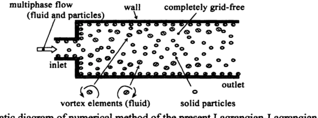
In the study by Iso and

Kmemoto9,

both fluid phase and particlephase

are

treated bythe

completely grid-ffee Lagrangian-Lagrangian simulation, without

use

of the Eulerian grids

as

schematically shown in Fig.6. It is possible to simulate directly particle motion oriented by

the vortex-induced fluid dynamical forces. Detail of the method and examples applied to intemal multiphase flows

are

described

in

the

paper

by Iso and

Kamemotol6.

Solid particles

were

treated by the $pa\hslash icle$ trajectory tracking method

as

a Lagrangian calculation.

Particle-particle and particle-wall collisions

aoe

calculated by adeterministic method. To $simpli\theta$the

problem in this study, the liquid-solid two-phase flows

are

treated

as

those ofdilute mixture

ofparticles and it is assumed that the effect of particles

on

the liquid flow is neglected

(one-way model). _And

a

solid particlesis considered

as

a

rigid sphere with

a

particlediameter.

Fig. 6 Schematicdiagram ofnumerical method of thepresent Lagrangian-Lagrangian simulation for intemal flows.

Based

on

the above assumptions, it is generally accepted that dominant forces

on

each

particle

are

the drag force, Magnus lift force, Saffinan lift force, force to accelerate the

virtually added

mass

in the ambient fluid, and gravitational force. The force on the particles

due to pressure gradient and the Basset force

are

neglected in this study. The equation of

motion for

a

particleisexpressed

as

$\frac{du_{p}}{dt}=\frac{1}{M_{p}}(F_{D}+F_{LM}+F_{IS}+F_{\nu^{r}M}+F_{G})$ ₍₅₎

Here, $u_{p}$ is the particle velocity vector, $M_{p}$ the particle mass, and $F$the force vector

on

the

particle; namely, $F_{D}$ is the drag force due to relative velocity of the particle to the fluid, $F_{LM}$

the Magnus lift force due to rotational motion, $F_{IS}$ the Saffinan lift force due to velocity

gradient, $F_{VM}$the force to accelerate the virtual added

mass

in the ambient fluid and $F_{G}$ the

omitted. They

are

similar to the formulas in the literature, for example, Tsuji et

al.17

and Yamamotoet al. 18

As the rotation of

a

particle is affected by the fluid viscosity, the equation of rotational

$particlerotationwhichistheoretica11yobtainedbyDenniseta1motionofeachparticleisnumerica11yso1vedbyconsiderin_{1}\S$

.

the

viscous

torque against

Particle-particle andparticle-wallcollisions

were

calculatedby

a

detemiinisticmethod. The traveling velocity and the rotational velocity ofa particle after collision

are

calculatedby the equations of impulsive motionof

a

particle. For the calculation of particle-wall collision, _the

collisionis modeled

as

irregular bouncing ofaparticle

on

the virtual wall model proposed by

Tsuji et

al.17,

in which the wall is replaced with a virtual wall having

an

angle relativeto the

real wall.

Physical motion of the particles is split up into two stages in order to reduce the computational load. Inthe first stage, all particles

are

moved based

on

the equation of

motion

without collisions. In the second stage, particle-particle collision is calculated, and then, the velocity of

a

particle after the collision is replaced with post-collision velocity without

changingtheposition.

In the beginning, the two-dimensional liquid-solid two-phase flow in a vertical channel

was

calculated to validate the coupled vortex element and particle method. The numerical simulation

was

performed for the

same

conditions

as

those in the two-phase experiments of Hishida et al. 20,

21.

The flow field is schematically shown in Fig.5. Flow direction of both

phases is downwards. The Reynolds number is $R_{e}=U_{c}W/\nu=5.0\cross 10^{3}$_, based

on

the

mean

velocity on the centerline $U_{c}=0.17m1s$ and the channel width $W=3.0x10^{-2}m$

.

Here, $v$is the

kinematic viscosity of water. Periodic boundary conditions for both phases were applied in

the streamwise direction due to restrictions

on

computational power. The length $L$ of the

computationalregion in the streamwise direction

was

equal to $3W$

.

Particles

are

introduced

into the channel using random numbers,

so

as

to satisfy uniform distribution at the loading

mass

ratio which is $m=1.1x10^{-2}$

.

_{Density and diameter of the particles}

are

$\hslash=2590kym^{3}$

(relativedensity: $\hslash/\rho_{f=}2.59$)and$d_{p}=500\mu m$, respectively.

$\ulcorner_{X}J^{r}$

A

Fig. 7 Schematic viewofliquid-solid two

phase flow in

a

vertical channel. Fig.velocities of8 The time-averagedfluid andsolid particles.streamwise

Figure 8 shows the results for the time-averaged streamwise velocities of fluid and solid

particles. In this downward flow, the particle velocity is faster than the liquid, because the

density of particles is larger. Numerical results showed very good agreement with the

quantitative accuracy and the applicability of the special combination ofvortex method and particletrajectorytracking method to intemal two-phase flow of high Reynoldsnumber.

Fig.9 Schematicview oftheliquid-solid two-phase flow

in

the mixingtee.

The coupled vortex element and particle method

was

applied to the two-dimensional

liquid-solid two-phase flowin amixing tee

as a

typical problem to mixing of liquid and solid

particles in ducts. The flow field is schematically shown in Fig.9. The flow field is not only the basic component in industrial pipelines but also the simple mixing device for multi-phase

flow. For details, refer to Kawashimaet $a1^{22,23}$and Blancard et

al.24.

InFig.9, the branchflow

merges into the main flow at

a

right angle. The cross-sections ofthe confluence

are

squares. The widths of themain and branch channels

are

$W_{1}$ and $W_{2}$, respectively, and the widthratio

is $W_{2}/W_{1}=0.5$ $(W_{1}=20 mm, W_{2}=10 mm)$

.

The volumetric flow rates in the main and branch

channels before confluence

are

$Q_{1}$ and $Q_{2}$, respectively, and the confluent flow rate ratio $Q_{2}/Q_{1}$ is changed

as

$Q_{2}/Q_{1}=1,2,3$, which correspond to the values of fluid momentum ratio $M_{2}/M_{1}$ of 2, 8, 18, respectively. The value of $Q_{2}/Q_{1}$ is controlled by changing only the

volumetric flowrate ofthe branch channel. The velocity

in

the

main

channel

is

$U_{1}=0.25m/s$,

and the velocity in the branch channel is $U_{2}=0.5,1.0,1.5n\vee s$

.

Reynolds numbers

are

$Re=(U_{3}W_{1})/v=1.0x10^{4},1.5x10^{4},2.0\cross 10^{4}$_, based on the average velocity $U_{3}$ and the width $W_{1}$ downstream of the confluent point. Here,$v$ is the kinematic viscosity of water. Particles

are

introduced into the branch channel only, using random numbers,

so

as

to satisfy uniform distribution at the volume concentration $C_{V}=0.01$

.

Density and diameter of particles

are

$\hslash^{=}$

2590 $kym^{3}$ (relative density: _{$\hslash/\rho_{f=}2.59$}) and _{$d_{p}=425\mu m$}, respectively. Direction ofgravity

is downward inFig.9.

$t$ $0$ ₁ a a _{5 7}

(a)Vortex elements (b)Fluidvelocity distributions

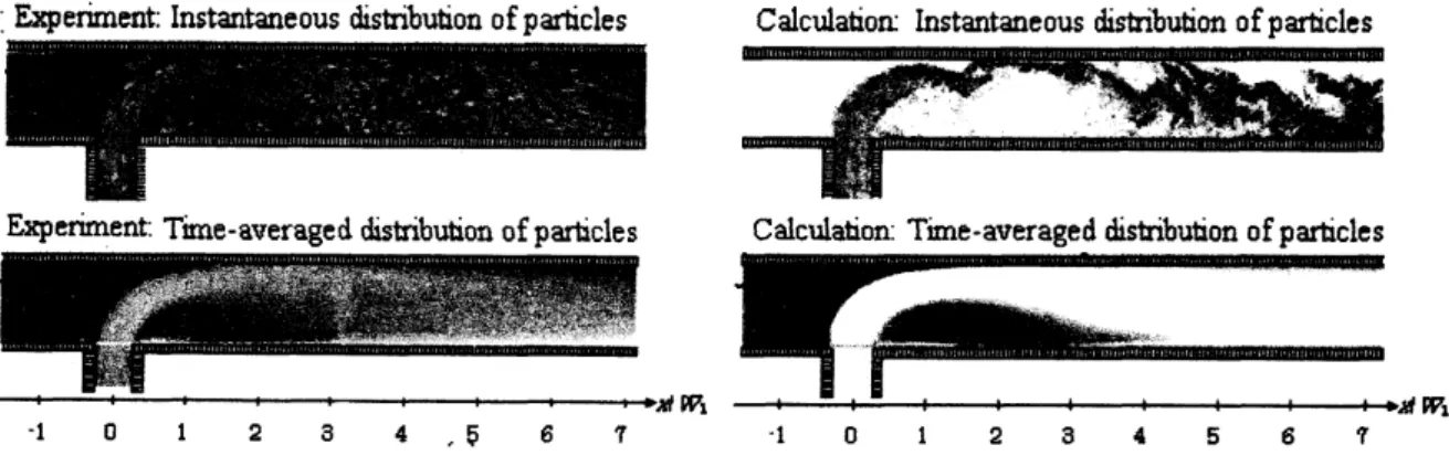
Fig.11 Comparisonbetween calculation andexperimentfordistribution ofparticles. Figure 10 shows two snap shots ofinstantaneous distributions ofvortexelements and fluid

velocity obtained by the numerical simulation. The condition of the confluent flow rate ratio is $Q_{2}/Q_{1}=2$, and the instantaneous non-dimensional times

are

_{$tUy’W_{1}=85.0$} and 87.5. The

contour of velocity expresses the streamwise fluid velocity. After two perpendicular flows merge in the mixing tee, the confluent flow deflects and unsteady flow separation

occurs

at

the downward

comer

ofthejunction. First,the confluentflowis accelerated inthe contraction region ofthe mixing point. Then, the flow is decelerated to the streamwise direction in the expansion. Consequently, unsteadyflow separation

occurs

andgrows up ffomthe bottomwall of themainchannel, _{because the adverse} pressuregradient is strong in the flow direction. The

separation vortices aggregate, break up and diffuse downward. Such phenomenon

was

also

obseivedin the experiments by inktracevisualization.

In Fig.11, the instantaneous and time-averaged distributions of solid particles for the condition of $Q_{2}/Q_{1}=2$

are

shown, and numerical results

are

compared with experimental

observations where thetime-averaged experimental photographs

were

taken by long

exposure.

Both, experimental and numerical results show that particleshave mixed almost unifornly at

$x/W_{1}=3$

.

As mentioned before, it is seen that the confluent flow deflected and the _unsteady

separations occurred at the downward

comer

ofthe junction. The confluent flow becomes

unsteady and complexdue tothe unsteadyseparation of flow from the channel walls. Thus, in

thecondition $Q_{2}/Q_{1}=2$, the abilityofthe particlemixingis good.

3.3 Plasma particletrajectorytracking method

Expanding the concept of the Lagrangian vortex method in which vorticity layers

are

expressed by

a

number of discrete vortex elements,

Ishimotol

and the group of the present

author have attempted numerical simulationofbehavior ofpure electron plasmain

a

magnetic field by introducing

a

number of chargedparticles called superperticles.

It is known that the motion ofnon-neutral plasma in

a

magnetic field is similar to the vortical flow offluid. So far, formation of coherent vortex structures of two-dimensional electron plasmas have been observed in experiments by $Kiwamoto^{25}and$ _{Sanpei et}

al26,

which

were

performed with the photo-cathode pure-electron plasma traps of

a

Malmberg-Penning trap type. The vortex crystal formation in two-dimensional plasma turbulence

was

theoretically investigated by Jin and

Dubin27

and for numerical simulation of the various phenomena in plasma, the particle-in-cell method, the leap-ffog method and others

are

explained byBirdsall and

Langdon28,

Naitou29,

Isiguro$3$

and

Ohsawa31.

The leap-ffog method

and Lagrangian method like the advanced vortex element method mentioned above is not

discussedindetail,

so

far.

In general, in a field with the intensity ofelectric field $E$ and the magnetic density$B$, the

motion of

a

charged particle with the strength of charge $q$ and the

mass

$m$ is expressed

as

follows.

$m \frac{du}{dt}=q(\Xi+u^{x}B)$

(6)

Here, $u$ denotes the velocity of the center of the particle which is given by $dr/dt$, and the

motion consistsofcircularmotion aroundthe axisof$B$and the motion of drifl inthe direction

of $E\cross B$

.

In the $rig\iota$-hand side of Eq. (6), the first temi $qE$ and the second $q(u\cross B)$

respectively correspond tothe Coulomb force and the Lorentz force acting

on

the particle. In the study, the two-dimensional motion of superpamcles of electrons in

a

uniform magnetic field $B_{o}$

was

calculated. Therefore, the intensity of electric field $E$ is calculated $fi\cdot om$ the

summation of individual intensity of electric field induced by each superparticle in the field and the magnetic density$B$is givenby$(B_{o}+dB)$ in which $dB$ denotesfluctuation ofmagnetic

density induced by motions ofthe electronic superparticles and it is calculated by the Biot-Savart law derived ffom the Maxwell equation. As the study

was a

firstattempt for the group of the presentauthorto apply the conceptofthe vortex method, asimple superparticlemodel

was

introduced, which has

a

spherical shape with the radius $r_{d}$ and the number of electrons

uniformly distributed in it is $N_{v}$ , and to simplify the numerical ffeamients, the effects of

electronic diffusion and collisions between particles

were

ignored. In order to compare the calculation results with experiments by

Kiwamoto25,

the

interaction

between two clouds of superparticles and the formation of vortex crystals ffom

a

ring cloud

were

calculated under the conditions similartothe experimental

ones.

$\sim$ .

$N1\bullet 253\bullet\bullet$

$\prime 1..\backslash \backslash _{\backslash \cdot=}:_{l^{\backslash }}..\dot{\alpha}_{\wedge^{\wedge}}^{:}\backslash ’..\cdot\cdot\cdot\cdot..\cdot.\cdot\cdot.\cdot$

$N|=5$ $\bullet\bullet$ $\infty$

$\oint_{\ddot{*}}$

, $-\backslash \cdot\sqrt{}\backslash ae_{:^{=}}\cdot..$

.

$0\mu\S$ _{$0.2\mu s$ $0.5\mu s$ $1.0\mu s$ $10.0\mu\S$}

Fig.12 Comparison ofcalculated results of merging of

a

pair of electronicplasma.

In the calculations ofinteraction between two clouds, the following conditions

were

used;

density of magnetic field $B_{o}=0.048N/Am$, the charge of

an

electron $e=1.6021$_xl$0^{-19}C$, the

mass

of

an

electron $m_{\epsilon}=9.109$lx 1$0^{}$ kg, the electric permittivity $a=8.8542$xl$0^{-12}C^{2}/(Nm^{2})$,

the electric perneability $\mu=1.2566x10^{6}N/A^{2}$_, the initial radius ofa_cloud $r_{i}=0.4$xl$0^{-3}m$, the

initial distance between two clouds $L=1.0x10^{-3}m$

.

_{In order to examine the effect of the}

numberofelectrons in

a

superparticle $N_{v}$and the imitial numberof superparticles in acloud$N_{i}$

combinations ofthe numbers

were

introduced

as

$(N_{v}=100, N_{i}=253)$ and $(N_{v}=460, N_{i}=55)$, and

three differentvalues for the radius ofsuperparticle

were

examined for each combination

as

$r_{d}$

$=2.5x10^{-5},$4xl$0^{}$ and2.5xl$0^{}$

$m$for the

case

$ofN_{i}=253$, and$r_{d}=5x10^{-5},$ 4xl$0^{}$ and5xl$0^{}$ _$m$

forthe

case

of$N_{i}=55$

.

The calculationtimestep

was

fixed

as

$d=1$_xl$0^{-10}s$

.

In Fig.12,

a

couple of calculation results of evolution of merging ofa pair of electronic

plasma clouds

are

shown, which

were

obtained for $(N_{i}=253, r_{d}\triangleleft-x10^{-7}m)$ and _{$(N_{i}=55,$}

$r_{d}$

$\triangleleft-x10^{7}m)$

.

From comparison of the results, it is clearly observed that

as

the time proceeds,

the two clouds catch and join each other, and then they finally merge into

a

new

isolated cloud due to the interactive motion of superparticles. The calculated evolution ofmerging is

in

qualitatively coincidence with the

experiments25.

And ithas been confirmed that there

are

no

significantdifferences inthe calculated merging processes correspondingtothe differences ofnotonly the numbers ofboth superparticles in

a

cloud and electrons in

a

superparticle, but also theradius of

a

superparticle,

as

far

as

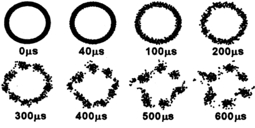
this studyis concemed.

Fig.13 $Fomat_{-}ion$of vortex crystal structure Rom

a

ring

In the calculation of the fomiationof vortex crystals ffom

a

ring cloud, the magnetic field conditions

are

the

same

as

those mentioned above. The initialouterradius and innerradiusof the ring cloud

are

$R_{o}=5\cross 10^{-3}m$ and $R_{i^{-}}\triangleleft x10^{-3}m$, respectively and the inner radius of the

conducting wall in which the ring cloud ofplasma

was

coaxially trapped is $R_{w}=5.5$xl$0^{-3}m$.

The number of superparticles in the ring cloud is $N_{r}=398$ and the number of electrons in

a

superparticle is $N_{v}=46$

.

In Fig.13, evolution of disturbance on motion of superparticls with

time and formation of six vortex crystals

are

clearly

seen.

It has been confirmed that the calculated features of vortex crystal formation is also in qualitatively coincidence with the experiments and numerical resultsreportedby

Kiwamoto25.

4.AView of NewDirection ofDiscrete Vortex Dynamics

In the former section,three examples ofapplicationsof Lagrangian trackingmethods based

on avortex elementmethod and aparticle method. It

seems

very interesting that although the

fluid is assumed

as

continuum and the particles

are

discrete ffagnents of

a

material, the

phenomena of vortex formation

are

certainlyobserved in dynamicmotionofboth

a

fluidand

particles. It is well known that the dynamic behaviors of statistically many particles like

powder, heavenly bodies inthecosmos,

cars

on a

crowdedroad, _and

_so

on,

_can

be represented

by the goveming equations in the fluid dynamics. So far, there exist such research fields

as

powder fluidization, ferrofluid, plasma flow,cosmic fluid,traffic flowand

so

on, and usually,

differential equations of fluid dynamics

are

appliedinto investigations ofthose

motions.

However, it must be considered that the applicability of those equations to

a

fluid dynamics

are

constructed formacroscopic flow fields on the assumption ofcontinuum.

Therefore, it is not always correct to introduce infinitesimally smaller size of grids in the

numerical calculation with use of a huge parallel-computer system aiming to increase accuracyofthenumerical treatnents.

As shown in the former section, it is important to consider that the introduction of

various

discrete elements is

a

key technology of the present numerical treamients, which is

common

to the calculations of both the dynamic phenomena ofvorticity transportation in

a

fluid and the dynamic motion of particles. In the vortex method, the discrete element is

a

discrete

vortex blob in which the distribution of vorticity and the particle size

are

modeled. In the

paiticle method used for the two-phase flow calculation, the discrete element is

a

solid particle itself in which

mass

and size

are

modeled. And in the particle method used in the plasma vortex calculation, the discrete element

consists

of

a

superparticle

in

which

a

distribution of electrons (mass and electric charge) and particle size

are

modeled. It

seems

a

stimulating fact for consideration of a

new

direction of discrete vortex dynamics that the

vortical phenomena not only in a fluid flow but also in

a

multi-particle flow

can

be analyzed

by the discrete element method. Although the presentauthor had considered the vortexblobs

to be ffagmentsto discretizethe continuous vorticity flield, recently he has looked them ffom a different point ofviewto be

a

sortofsuperparticles, which essentially consists ofa number

ofelementary particles. Therefore, it will be very interesting to accumulate comprehensive

knowledge on various kinds of vortex motions Rom molecular dynamics to cosmetic flowby

investigating the fiactal features of the vortex motion and by modeling superparticles with various scalesand characteristics requiredin corresponding dynamic fields.

5. Conclusions

In this paper, aiming to overview the recent attempts of progressive application ofthe advanced vortex method, _{mathematical background and numerical} procedure of the method

aoe

briefly explained, and characteristic results of the progressive studies

on

simulation of complex flows around a 100 $m$ runner, liquid-particle two phase flows in

a

channel and

vortical motion of plasma clouds in

a

magnetic field

are

digested with explanation ofthe particle methods used in the latter two studies. And finally,

a new

direction of further

developmentofthediscrete particle methods forvortex dynamuics is discussed. The discussion

issummarized

as

follows.

1$)$ The three examples of applications of the vortex method, the coupled vortex-particle

method and the plasma particle method,

_seem

to suggest that most of the vortex motions observed in various fields

are

essentiallyorientedto the discrete particledynamics instead

ofthecontinuousfluid dynamics.

2$)$ It is not always correct to introduce infinitesimally smaller size of grids inthe numerical

calculation with

use

of

a

huge parallel-computer system aiming to increase accuracy of the numerical treatnents, because the molecular dynamics govems the microscopic field insteadof the continuumdynamics.

3$)$ Considein

$g$ the above discussion, it

seems

interesting to accumulate comprehensive knowledge

on

various kinds ofvortex motionsffommolecular dynamicsto cosmetic fluid

dynamicsbyinvestigating the ffactal features.

4$)$ It will be a

new

direction ofexpansion ofthe concept of discrete elements methods to

establish comprehensive algorithms of modeling physical behaviors of elementary

particles like vortex blobs and plasma superparticles which have various scales and

ACKNOWLEDGMENTS

The author wishes to thank Dr. Ojima of CMH for discussing on the treatment ofdiscrete

vortex particles and providing with the software of vortex method used in the calculations of

flows around

a

$100m$ runner, and Dr. Iso of_IHI for _discussing

on

_{application of the panel}

methods forintemalflows. REFERENCES

[1] Leonard, A., Vortex methods for flow simulations. J. Comp. Phys. 1980, 37,

289-335.

[2]Sarpkaya, T., Computational methods with vortices-the 1988 Freeman scholar $1ecmre_{0}$

J FluidsEngng., 1989, 111, 5-52.

[3] Kamemoto, K., On attractive features of the vortex methods. Computational Fluid

Dynamics Review 1995, ed. M.Hafez and K.Oshima, JOHN WILEY $\backslash$

&SONS,

1995,

334-353.

[4] Kamemoto, K., Recent$con\theta ibution$ of

an

advanced vortex element method to simulation

ofunsteady voitex flows. ComputationalFluid$1\eta namics$ Journal, 2007, $15(4):55,422-$

437.

[5] Ojima A. and Kamemoto, K., Numerical simulation ofunsteady flows around

a

fish. Proc.

_of

the Third International

_Conference

on

Vortex Flows and Vortex

Modets-ICVFM2005, Yokohama, Japan,November2005,96-101.

[6] Greengard L. and Rohklin V., A fast algorithm for particle simulations. J Comp. Phys. 1987, 73-2,

325-348.

[7] Fukuda K. and Kamemoto, K., Application of

a

redistribution model incorporated in

a

vortexmethod to turbulent flow analysis. Proc.

_of

the Third International

_Conference

on VortexFlows and Vortex Models-ICVFM2005, Yokohama, Japan, November2005,

131-136.

[8] Kamemoto K. and OjimaA., Application of

a

vortexmethodto fluiddynanuics insports

science Proceedings

_of

FEDSM2007 5th Joint $ASME/JSME$ _{Fluids Engineering}

Conference,July30-August2, 2007 San Diego,Califomia, USA,FEDSM2007-37066.

[9] Iso Y. and Kamemoto K., Vortex method and particle trajectory tracking method for

Lagrangian-Lagrangian simulation applied to internal liquid-solid two-phase flows. Proc.

_of

the Third International

_Conference

on Vortex Flows and Vortex

Models-ICVFM2005, Yokohama, Japan,November2005, 287-292.

[10] Ishimoto S., _{Application of vortex method into motional simulation of plasma particles.}

Bachelor Thesis, _{Yokohama National University, Submitted to Prof.} Kamemoto,

February

2007.

[11] Wu J.C. and Thompson J.F., Numerical solutions of time-dependent incompressible Navier-Stokes equations using

an

integro-differential formulation. Computers 6}Fluids,

1973, 1-1, 197-215.

[12] Uhlman, J.S., An integral equation fomulation of the equation of motion of

an

incompressible fluid. Naval Undersea

_Warfare

Center, 1992, T.R. 10-086.

[13] Ojima A. and Kamemoto K., Numerical simulation of unsteady flow around three dimensional bluffbodies by

an

advanced vortex method. JSME Int. Journal, B, 2000,

43-2, 127-135.

[14] Winkelmans G. and LeonardA., Improved vortex methods forthree-dimensional flows. Proc. Workshop

on

MathematicalAspects

_of

Vortex Dynamics, Leeburg, Virginia,USA,

1988, 25-35,

[15] Nakanishi Y. and Kamemoto K., Numerical simulation of flow around

a

sphere with vortexblobs.Journal WindEng. andInd Aero, 1992,46-47, 363-369.

[16] Iso Y. and Kamemoto K., Vortex method and particle trajectory tracking method for

liquid-solid two-phase simulation applied to intemal flows. Trans. JSME Ser.B, 2005,

71-71, 2671-2678, (inJapanese).

[17] Tsuji Y., Morikawa Y., Tanaka T., Nakatsukasa N. and Nakatani M., Numerical simulation ofgas-solid two-phase flow in

a

two-dimensional horizontal channel. Int. $J$

MultiphaseFlow, 1987, 13-5, 671-684.

[18] Yamamoto Y., Potthoff M., Tanaka T., Kajishima T and Tsuji Y., Large-eddy

simulation of turbulent gas-particle flow in

a

vertical channel: effect of considering inter-particle collision. J FluidMech., 2001, 442,

_303-334.

[19] Dennis, S. C. R, Singh S.N. and Inghan D.B., The steady flowdue to

a

rotating sphere

at lowand moderate Reynolds number. J FluidMech., 1980, 101, 257-279.

[20] Hishida, K., HanzawaY., SakakibaraJ., Satou Y. and MaedaM., TransofJSME, Ser. $B$

1996,62-593, 18-25 (in Japanese).

[21] Hishida, K., HanzawaY., SakakibaraJ., Satou Y. andMaeda M., Trans ofJSME, Ser. $B$

1996, 62-593,26-33 (inJapanese).

[22] Kawashima Y., _{Nakagawa M. and Inoue} S., Characteristics ofmixing due to confluent

flow in

a

two-dimensional right-angled T-shaped flow section. The Society

_of

Chemical

EngineersJapan, 1982,8-2, 109-114,(in Japanese).

[23] Kawashina Y., Nakagawa M. and Inoue S., Flow pattems at

a

two-dimensional

right-angled T-shaped confluence. The Sociely

_of

Chemical Engineers Japan, 1982, 8-6,

664-670, (in Japanese).

[24] Blancard J. N. and Brunet Y., Interaction between

a

jet getting out of

a

tluin slit and emerging into

a

crossflow.ASMEFluids Eng. Div. Conf, 1996, 4, 39A6.

[25] Kiwamoto Y., Vortex dynamics in nonneutral plasma. J Physical Society

_of

Japan,

2001,56A, $253- 261$, (inJapanese).

[26] Sanpei A., Ito K., Soga Y., Aoki J. and Kiwamoto Y., Formationof

a

symmetric vortex configurationin

a

pure electron plasma trapped with

a

penningtrap. Hyparfine Interact,

2007,

_174.71-76.

[27] Jin D.Z.and Dubin D.H.E., Theory of vortex crystal formation in two-dimensional turbulence. Phys. Plasmas,2000,7-5,1719-1722.

[28] Birdsall C.K. and Langdon A.B. , Plasma Physics via Computer Simulation

(McGraw-Hill Book Company, NewYork, 1985 and Adam Hilger, Bristol, Philadelphia and New

York, 1991).

[29] Naitou H., Basic theory of particle simulation. Jr. Plasma and Fusion Research, 1998,

74-5, 470-478 (in Japanese).

[30] Ishiguro S., Electrostatic Particle Simulation. Jr. Plasma andFusion Research, 1998, 74

-6, $591- 597$(in Japanese).

[31] Ohsawa Y., Relativistic Electromagnetic Particle Simulation. Jr. Plasma and Fusion