第 55 卷 第 2 期
2020 年 4 月
JOURNAL OF SOUTHWEST JIAOTONG UNIVERSITY
Vol. 55 No. 2
Apr. 2020
ISSN: 0258-2724 DOI:10.35741/issn.0258-2724.55.2.5
Research article
Mechanical Engineering
A
S
IMULATION
M
ODEL TO
I
MPROVE
P
RODUCTIVITY IN THE
P
IPE
M
ANUFACTURING
I
NDUSTRY
提高管道制造行业生产率的仿真模型
Rabia Almamlook a, Harith M. Ali b, *, Arz Qwam Alden b, Anad Afhaima c, Faieza Saad Bodowara c , Sahapol Hoon Knew a
a Department of Industrial Engineering, Western Michigan University Kalamazoo, Michigan, USA, rabiaemhamedm.almamlook@wmich.edu
b Mechanical Department, Engineering College, University Of Anbar Ramadi, Al-Anbar, Iraq, eng.harith85@uoanbar.edu.iq, arzrzayeg}@uoanbar.edu.iq
c
Department of Chemistry, Institute of Technology, University of Florida Gainesville, Florida, USA, faiezabodowara@yahoo.com
Received: June 07, 2019 ▪ Review: September 19, 2019 ▪ Accepted: February 15, 2020 This article is an open access article distributed under the terms and conditions of the Creative Commons Attribution License
(http://creativecommons.org/licenses/by/4.0)
Abstract
Improving productivity in the pipe manufacturing industry is a major challenge that manufacturing companies in contemporary competitive markets face. The purpose of this study was to improve productivity in the pipe manufacturing industry by applying manufacturing principles that employ simulation modeling. An approach to improve productivity which focuses on the process of workstations and workforces was proposed . The proposed approach’s target was to boost the productivity of providing clients’ prerequisites and leaving a few products in the store for other clients. A simulation model based on the data collected from the steel pipe company, Bansal Ispat Tubes Private Limited’s in India, was used to improve its operational performance. The research methodology included a pro-simulation model, suitable distribution and investigating data. The simulation model was created by simulating each work station and assessing all relevant processes depending on the collected data. The real job-shop data was collected from the machinery production line and supervision workers with observations made during the manufacturing process. The techniques used include videotaping of the operation, interviewing liber by a video camera. The best continuous distributions were choose to achieve a suitable statistical model. The outcomes maybe contribute to improving the productivity of the manufacturing industry. Moreover, the results might help solve scheduling problems in modeling and simulating pipe manufacturing, revealing effective strategies to increase productivity in pipe manufacturing. Thus, the findings could encourage healthy competition between businesses and industries.
摘要 在当今竞争激烈的市场中,制造公司面临的主要挑战是提高管道制造行业的生产率。这项研 究的目的是通过应用采用模拟建模的制造原理来提高管道制造行业的生产率。提出了一种以工作 站和劳动力为重点的提高生产率的方法。拟议方法的目标是提高提供客户必备产品的效率,并在 商店中为其他客户留一些产品。基于从印度班萨尔钢管私人有限公司的钢管公司收集的数据建立 的仿真模型用于改善其运营绩效。研究方法包括模拟模型,适当的分布和调查数据。通过模拟每 个工作站并根据收集的数据评估所有相关过程来创建模拟模型。实际的车间数据是从机械生产线 和监督人员那里收集的,并在制造过程中进行了观察。所使用的技术包括对手术进行录像,通过 摄像机采访解放者。选择最佳连续分布以实现合适的统计模型。结果可能有助于提高制造业的生 产率。此外,结果可能有助于解决建模和模拟管道制造中的调度问题,从而揭示提高管道制造生 产率的有效策略。因此,研究结果可以鼓励企业和行业之间的健康竞争。 关键词: 仿真模型,专业模型,生产率,管道制造行业
I. I
NTRODUCTIONIn the competitive world, businesses and industries have to improve their performance to retain themselves. Low-efficiency is one of the several challenges faced by manufacturing companies in competitive markets. Bansal Ispat Tubes Private Limited’s presence in one of the largest steel markets in India required effective production planning to improve the production procedure to achieve increased competence [1]. The final product plays a crucial role in ensuring the success of the operation in production processes, since it could be applied to define the higher quality of the available product. Owing to higher quality requirements along with the increased demand for the products, the company management considered various ways to improve the all line production. The increase in customer demand has caused several problems in the production of the pipes. Scheduling work is one of these problems. Therefore, additional shifts have been added by the pipe manufacturer to increase production. These additional shifts resulted in an increase in the work-in-process, which leads to further bottlenecks in the line of
manufacturing. Moreover, operational
effectiveness with minimal cost is affected by maintenance policies [2]. To meet the demands of the market, the companies' tried to improve productivity and increase production. Modelling and simulation techniques of manufacturing may help to create an understanding of the processes and can also assist in identifying and testing strategies that lead to maximum efficiency in production [3], [31]. The possibility of accurate identification of all inputs and outputs in the form of financial value highly impacts the process of constructing the productivity measurement model [4]. Also, the performance is identified as a critical success factor related to the company.
Therefore, there are several types of simulation modelling software that exist in the market to improve and develop complicated manufacturing systems [5], [6], [7], [8], [9], [10], [11], [12], [13].
For decades, modelling and simulation have been employed by companies worldwide to improve the design, evaluation, and development of the operation of complicated systems [11], [14], [15]. Many industries and businesses require effective production planning to improve their performance to retain their businesses in the competitive world. Performance could be used to specify product availability and increase quality. Therefore, performance plays a crucial role in ensuring the success of the operation for the
production processes company [16]. The
modelling and simulation software called pro-model has grown to be a useful tool for numerous applications in real-world engineering [17], [18], [19], [20]. The pro-model designed to model manufacturing systems is applicable from small job workshops and machining cells to large mass production and supply series systems [21], [22]. Discrete simulation modelling can also be applied to improve productivity [23]. The advantages of utilizing discrete-event simulation have been the focus of several studies [5], [17], [20], [24], [25], [26], [27], [28], [29].
These studies have identified the benefits of using discrete-event simulation such as systems deviation level, changes in system performance, and effects of changing process variables including labour and machines. Thus, this study aimed to increase the quantity of production and simulate the time that is required to achieve customers' requirements, while leaving some stock in the warehouse for new customers. A pipe manufacturer in India was modelled to increase line production by decreasing direct labour hours per machine. Furthermore, the model can assist in understanding processes, decisions, and resources.
The model can also help in identifying and examining the strategies that increase production efficiency.
II. A
PPROACH ANDM
ETHODOLOGYA. Background on the Manufacturing Steel Pipe Company
The manufacturing line consists of two major processes consisting of the slitting process and conversion process to manufacture finished goods. There are three main entities associated with the manufacturing of the Mild Steel (MS) pipes. Also, they use mother coil steel as the raw material, slatted coil as the intermediate material, and the different sizes of the pipes are the final product that will be stored and delivered to customers.
To manufacture the pipes, other essential tools were also used as entities for the process to be complete. The first process, which is slitting,
consists of seven locations, one operator, one foreman, and four full-time labour. It involves three entities such as mother coil, slitting tool, and silted coil. The second process which is the conversion to pipes consists of sixteen locations, one operator, one foreman, and six full-time laborers. It involves five entities such as silted coil, stamps, welding rolls, deburring tools, and MS pipes. The process needs to run at a specific speed and a certain amount of heat for the welding. To change it to a different type of material it takes twelve hours of change time and a large amount of scrap is subsequently generated. Therefore, one type of material is completed first. The company runs for twenty-four hours a day with three shifts that are eight hours each.
B. Identify Components and Analyse the Model
A working Pro Model simulation model contains the following elements Table 1.
Table 1.
Elements of Pro Model simulation model
C. Collecting and Analysing Data
All information available throughout this study were claimed by the supervision workers. Data collected throughout this study are
identified the times of admission, dynamic symbol reports, quick response interferences, and expulsion was needed to estimation deterioration probabilities, charges, and products. The results
involved cycle times of machine workers, the number of clienteles, in both system and line, dispensation times, and capitals downtime. Subsequently, the model was constructed, the simulation was in progress to define the suitable of fit of a statistical model. Furthermore, some of the decision factors which were including the travel distance between locations, allocation of the workforce, skills and expertise of the workers,
operating environment and temperatures,
machines number in the system and speed of the tools setup were implemented.
D. Method for Collecting the Data
The data is collected from a Real-Life System, which is manufactory of pipe. We collected real job-shop data from the Machinery production line with observations made during plant. The techniques used include videotaping of the operation, interviewing liber by video camera. This type of data is very important in creating the simulation model. Therefore, to be able to get all
the data required to perform the simulation, the first step to collect date was Building the Excel Data File. The Excel data file consists of one
spreadsheet. This spreadsheet contains
information about the manufacturing processes that take place on the Manufacturing. After that we have started with collection date.
As the process is a continuous process so we have some run time which is not collected as the part of this experiment. The data collected is shown for the first 30 observations of each element respectively. For instance, one mother coil produces 6-8 slitted coils, to Produce 30 slitted coils we need only 4-5 coils max, so to have the data much more information we divided into 2 different processes and the Data Collection process is also different respectively. The first 30 customers regardless of what material it is shipping. The slitting process and conversion Process consists as shown in Tables 2 and 3, respectively.
Table 2.
Slitting process consists of 4 major elements
Table 3.
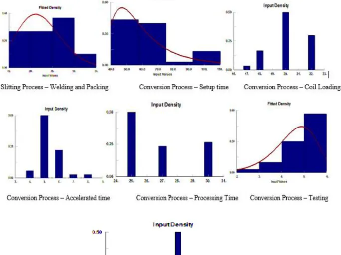
E. Appropriate Distribution
To get a suitable statistical model, the best continuous distributions to fit the input information, investigate maximum likelihood assessments for those distributions, exam the outcomes for the goodness of fit, and demonstration the distributions in the instruction of their comparative rank were choose.In this study, each station and product with their respective times was presented successfully. It was observed utilizing a tool called Stat Fit was one of the serious steps to program simulation using Pro-Model and the technique used to procedure all the information. Describing the
distribution of process waiting time in each procedure was required. All needed information could be input in this tool, and it could process and examine throughout all the different functions to select the statistical function that best fits input data. Then it provides the descriptive information from the data and more illustrative information, such as graphics and scatter plots, as shown in Figure 1. As can be seen in the figure,
the observations are independent of all
distributions selected for each process. The collected data for the setup time before running the slitting process seems to fit.
Figure 1. Process flow chart of MS pipe manufacturing model
The collected data for this process does not fit any built-in discrete and continuous distributions so, a user-defined distribution is preferable. Whereas a good rank typically shows that the
fitted distribution is a good demonstration of the input data, an absolute indication of the goodness of fit is also known as shown in Table 4.
Table 4.
Procedures and chosen distributions
III. R
ESULTS ANDD
ISCUSSIONA. Model Application with Pro-Model
The simulation model is built depending upon a full list of assumptions. To manufacture finished goods, the line of manufacturing includes two essential processes which are the
slitting process and conversion process.
Moreover, there are five main entities are associated with MS pipes manufacturing. The first step is to build several locations containing buffers, machines, conveyors further, and workstations. The locations include four full-time laborers, an operator, and a foreman. Also, the locations have three entities which are mother
coil, silted coil, and slitting tool. The conversion to pipes is represented in the second step and it is consisting of a foreman and six full-time laborers. Also, this step involves five entities which are welding rolls, stamps, the silted coil, MS pipes, and deburring tools. For the welding, the process has to turn on at a determined speed at a particular amount of heat. The company works for 24 hours/day with three shifts, each shift works eight hours. The entities are described in the third step. The entities include raw materials, loads, piece parts, finished products, assemblies, operators, orders, machines, pipes, and labels. The fourth step is represented by building the entities' arrival patterns. The fifth step includes developing the model which is employing additional resources and consistent path networks that are required to transfer entities among locations.
B. Verification and Validation of Simulation Model
Before initiating the validation study, the engineers and the firm owners were consulted to obtain all the information required to fully
describe the actual production processes. It was uncovered that the processes should include two lines, to increase productivity. As this is not practical, the simulation model was an alternative solution. The simulation was thus based on the monthly estimated requests for dissimilar products. The model was validated by (1) monitoring production line behavior , (2) examining the output/statistics, (3) utilizing "debug" and "trace" software tools, and (4) conducting a code/model review.
1) Simulation Model Verification
The model structure was developed by simulating each work station and assessing all relevant processes. Next, the model was debugged and its ability to recognize errors in work procedures was assessed. Several issues were identified, as discussed below.
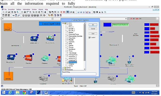
a) Pipes Accumulation at Warehouse 4
All produced pipes should be shipped directly to the customer. Practically, the "watch the animation for correct behaviour" and "trace” software tool showed that is not practical to accumulate up to 300 pipes once.
Figure 2. Using trace facilities with the software
b) Utilization of the Location “Weightier” Was Zero (0)
We used 2 mm, 3 mm, and 4 mm pipes. By using the method "Checking for reasonable output/statistics," we determined that we were not using the weighing machine. The customer’s vehicle had to wait for some time to record the weight of the purchased pipes for accounting purposes. This was
observed by using the second technique: checking for reasonable output/statistics.
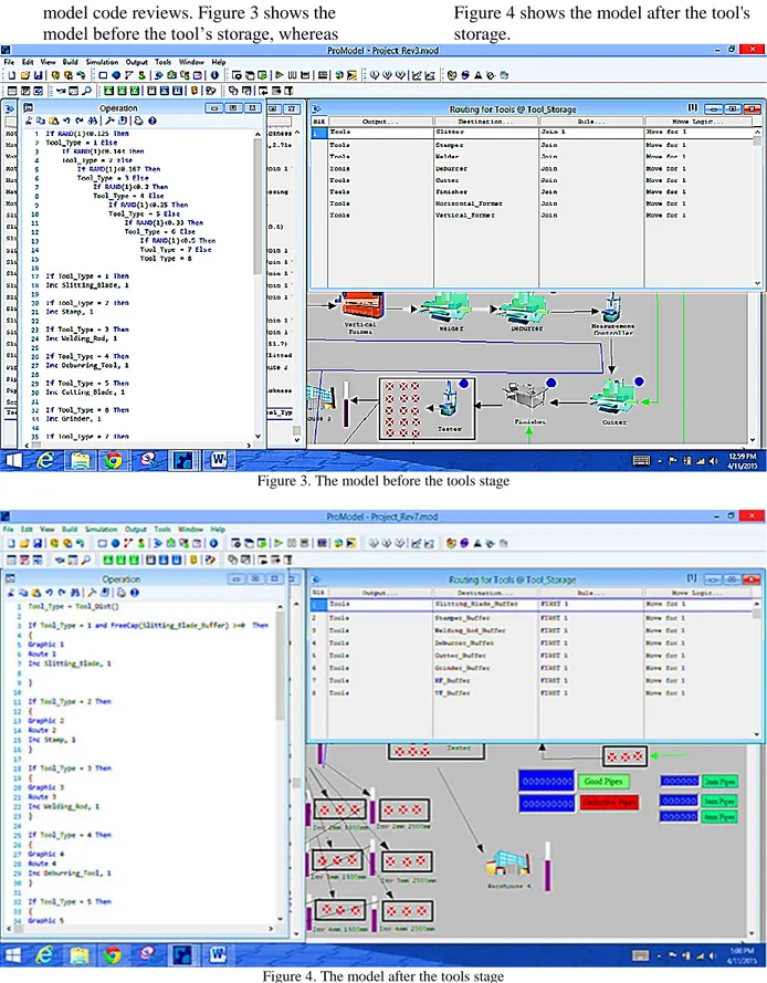
c) For the Tool Storage, We Changed the Command
The command rand () 8 to 9 times was used which made more complicated and the results had only minor changes. User-defined functions and tables to assign attributes for each type of tool were utilized. These had been used to conduct
model code reviews. Figure 3 shows the
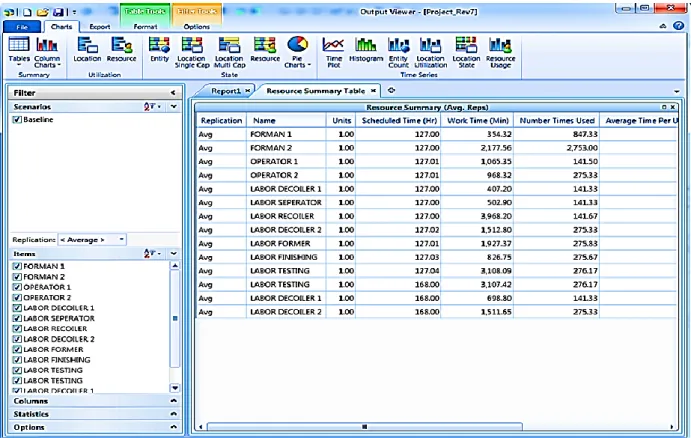
model before the tool’s storage, whereas Figure 4 shows the model after the tool's storage.
Figure 3. The model before the tools stage
Figure 4. The model after the tools stage
d) Using Two Labourers/Workers at One Location
At some locations, we used two labourers since the job cannot be done with just one worker in real life; we were unsure how to
use 2 labourers for one location using the “use” command. We changed that to the get > use > release command. Figure 5 shows the model after the changed labour command.
Figure 5. The model after the tools stage
e) Different Lengths of Pipes Not Included
Previously, at the cutter location, each length difference, including 750mm, 1000 mm, 1500 mm, and 2000 mm, was not assigned to each pipe, which was a problem; this issue was rectified by using the debugging tool.
2) Validity of the Simulation Model
The results of this simulation are comparable to an actual life situation because this study simulates a process that already exists. A model's validity can be investigated by determining the resemblance between the outcomes of the simulation and those of the real system. Thus, to determine the validity of our model, a confidence interval test for each station was performed and compared with real-life values. In this way, the validity was determined by following the running time for each product at each station. Comparing the results of a real-world system with a simulation model is considered a reliable approach. The process of validation is as follows:
• Based on the time-series plot on the output, the model required a warm-up period of around six weeks to reach a steady state. Data collection began in the 7th week and weekly validated results were obtained, including throughputs and Wished in pipes (WIPs).
• The simulation model was run using historical input data. The experiments involved running six replications of the process before making the necessary calculations.
• The calculations used statistical methods to compare the real-world data with that from the simulation. The confidence-interval approach was used to compare the data of the real-world system with the simulation results.
Tables 5 and 6 show the performance confidence and WIP for the pipes (good and bad). Confidence-interval testing was done for 750 mm, 1000 mm, 1500 mm, and 2000 mm pipes and used the number of weekly good pipes (thickness = 2 mm, 3 mm, and 4 mm). In most analyses, an alpha of 0.05 was used as the cut-off for significance. Since the p-value was more than 0.05, we accepted the null hypothesis (H0) that there was a difference between the means and concluded that a significant difference does not exist. If the P-value was less than 0.05, the null hypothesis had to be rejected. The observations of the input and output of random variables in the system and the model were statistically identical. Since we accepted H0, we tentatively accepted the model as valid. This approach resulted in the model and system outputs being positively correlated. The members of the project team ensured that the models were sufficiently accurate.
Table 5.
Table 6.
WIP for pip (good & bad)
C. The Design of the Experiment
This paper documents experiments using a simulation model and the statistical analysis of the output from the simulation runs. The simulation model in this study can be classified as a non-terminating simulation of the general manufacturing processes. Thus, the experiments were conducted by running multiple replications of the period of interest. Trying many ‘what-if’ scenarios based on output interpretations, such as the percentage of resource idling time, percentage of each entity blocked in each process, etc., leads to too many experimental results. In order to reduce the number of experimentations, each factor was studied and the tasks related to each factor were identified. The different parameters and run simulations were carried out on the scenario manager in order to check whether the throughput was improved. Eventually, the following three main scenarios that may have affected the weekly throughput were ended:
Policy 1: Increase in the conversion process capacity from 1 to 2.
Policy 2: Increase in the raw material arrival rate from every 96 hours to every 48 hours.
Policy 3: Both policies were
implemented simultaneously.
The process was non-terminating. The simulation was allowed to run for some time before the output on the time-series plot was interpreted to determine when we needed to start collecting the weekly throughput. The system ran at a steady rate from the 7th week onward, indicating that the simulation had a six-week warm-up period. The batch-means method was used to split the data from weeks 7 to 17 into their corresponding weeks, as in the real system.
The baseline model, as well as three additional models implemented with three policies, were run to observe the effects on the weekly number of the passed the MS pipes. We used ten replications of weekly throughput for each scenario for the design of experiments output analysis. Subsequently, we started with a simulation output analysis phase. Here, three scenarios were considered that were suspected to have some positive effects on the throughput, as shown in Table 7. To validate the base model and to prove its accuracy, simulated modelling runs were applied. The validation process of the current base model was specified by comparing the company’s actual productivity to the base model simulation’s productivity, as shown in Table 7. This test verifies that the H0 for averages are equal:
H0: μ1 -μ2 = 0 H1: μ1 -μ2 ≠ 0
with 95% confidence, and the consequences show that there is no significant difference between the real system and the simulation model. The statistics were applied by using ten weekly evaluations.
Table 7.
Scenario of simulation data
IV. E
XPERIMENTALR
ESULTS ANDD
ISCUSSIONThe experiment method is applied for designing scenarios and the method of full factorial. Numerous factors were measured, and it was statistically determined if those factors had an effect on the weekly number of good pipes. The model was examined to discover possible impact factors, and we discovered that the
throughput of good pipes is a crucial variable in the output. Therefore, it is important to improve the throughput of good pipes in order to significantly improve the system output. The model was simulated in such a way as to determine the amount output within a given amount of time. This was achieved by using various inputs. Then the outputs were compared to choose the model that produces the highest productivity.
A. 2-Way ANOVA
In this study, 2-way ANOVA was used to determine the significant factors and interaction among A and B on the response variable, and paired t-tests were used for the baseline model and the three scenarios. Table 8 demonstrations that p-values for interaction between Mother Coil Arrival Rate and Conversion Process Capacity equal to 0.67 which is greater than 0.05. Therefore, all suggestions for the difference have ineffective to be excluded.
Table 8.
Results of 2-way ANOVA
The statistical outcomes show that there is no significant difference between the Mother Coil Arrival Rate and Conversion Process Capacity and. Also, the results reveal that the combined models, Mother Coil Arrival Rate, and Modelling Conversion Process Capacity have great impacts on the simulation outcomes.
Moreover, both simulation models produce similar simulation outcomes [30]. These results lead to an understanding that there is no significant evidence between the factor of Conversion Process Capacity and interaction of Mother Coil Arrival Rate. So, the null hypothesis fails to reject. These results would lead us to retain H0 and conclude that there is no significant evidence for a supplement that there is the interaction between factor Conversion Process Capacity Factor Arrival Rate of Raw Material interaction since p-value = 0.67 is greater than α = 0.05), so we fail to reject the null hypothesis. Likewise, since F = 0.188 < F critical, then fail to reject Ho. (See the interaction plot). To test the main factors.
Figure 6. Interaction between factor Conversion Process Capacity (A) and factor Arrival Rate of Raw Material (B)
1) Hypotheses: (Conversion Process Capacity) Ho: Main factor conversion process capacity
is not significant.
Ha: Main factor conversion process capacity
is significant.
P-value = 0.78 > 0.05, we failed to reject the null hypothesis and concluded that there is strong evidence that the main factor Conversion Process Capacity is not significant. In other words, the conversion process capacity does not statically affect the throughput.
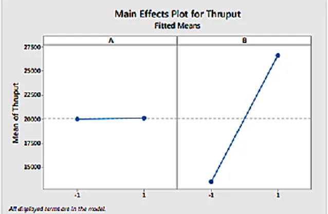
It can be noted that F equals 642.21 and the p-value equal zero is lesser than the importance level. Subsequently, the p-value equal is zero and less than 0.05, we excluded the null hypothesis. There is a significant effect of the main factor Arrival Rate of Raw Material on the response. Consequently, hypotheses must be excluded and achieve that there is a significant difference between the interaction of the Arrival Rate of Mother Coil and Conversion Process Capacity productivity, as shown in Figure 7. Thus, there is an important outcome of the main factor Arrival Rate of Mother Coil on the response.
Figure 7. Main effects between factor Conversion Process Capacity (A) and factor Arrival Rate of Raw Material (B) B. Paired t-Test: Two Sample
(Supplementary)
An initial number of replications of 10 was used for the simulation runs in Pro-Model Compared with the current or baseline model, each scenario while assuming a confidence level
of 95% is as follows. Table 9 shows a comparison between the baseline model and each scenario. At the alpha level of 0.05, P-value 0.620 > 0.05. Then we failed to reject Ho and conclude that there is no significant difference between the throughput of the baseline model and policy 1 implementation. Thus, to start with the first scenario, hypotheses must be rejected and determine that there is a significant difference between the productivity of the baseline model and the first of the Scenario. In scenario 2, at the alpha level of 0.05, P-value 1.96082E-09 < 0.05. Then we rejected Ho and concluded there is a significant difference in the throughput of the baseline model and the model after the policy 2 implementations while as in scenario 2, at the alpha level of 0.05, P-value 1.08829E-09 < 0.05. Then we rejected Ho and concluded there is a significant difference in the throughput of the baseline model and the model after the policy 3 implementations.
Table 9.
Comparison between baseline model and each scenario
However, the second and third scenarios
demonstrated that the hypotheses have
unsuccessful to be rejected and conclude that there is no important variation between the baseline model productivity and the model’s scenario (second and third). The simulation forecast that the productivity of the general system improves, and the production average rate rises. The model for the proposed scenario was simulated in order to ensure that the system reached a steady state. Furthermore, the stable state was recognized after the ten-week period of running production. The results illustrate that there is a variation between the conversion process capacity, productivity, and interaction of the mother coil arrival rate. Thus, the company must increase the rate of arrival to ameliorate productivity in the absence of increasing the conversion process capacity. Furthermore, it displays that the simulation of conversion process capacity, mother coil arrival rate, and combined models influence the simulation model results, and both models yield an identical simulation result.
V. C
ONCLUSIONIn this paper, we have presented a case study
on improving productivity in a pipe
manufacturing industry. What modern simulation software tools can achieve is to afford solutions for improving the productivity of the current manufacturer schemes by ascertaining the performance of the system. Thus, possible improvements inside the production line were recognized and applied in an improved scenario model. This study has established that the amount of current production might not meet the demand for the next few years, and that, as a result, the company only needs to increase the arrival rate to improve productivity. The study has also shown that the simulation technique could be employed by using a computer, which would assist in decision making. The simulation models have suggested a significant improvement in the
throughput of manufacturing. We would
recommend increasing the arrival rate only, and improving productivity without increasing the conversation process capacity associated with some large amount of investment based on the simulation model, even though the company is now manufacturing steel pipes according to its capacity. Furthermore, in order to meet the project objective, it will be necessary to negotiate with the raw material supplier and to conduct a feasibility study of the capacity increase. The limitation of this study is that the scenarios have only focused on improving the productivity of the manufacturing system, whereas some additional important factors, such as minimizing the waiting time, should also be considered. Future studies must focus attention on recognizing the problems of each subsystem, such as downtimes that are associated with labor-intensive operations—e.g., an operator starting his shift late or an operator finishing his shift early—and must devise solutions to develop the manufacturing process.
In conclusion, therefore, this study enables managers to gain a wider perspective on the ability to simulate complex systems, and to present alternatives to improve the process, which will provide strong forecasts for future manufacturing. The study concludes that the arrival rate of the mother coil to the warehouse significantly affects the throughput. In general, the study also shows that the application of manufacturing principles with the help of the simulation model could add significant value to the establishment and increase of operational productivity. This work can be easily modified or adapted to other industrial businesses in order to identify the inefficiencies in the manufacturing procedure.
A
CKNOWLEDGMENTThe authors received no financial support for the research and/or publication of this article.