ISSN -
0258-2724 DOI
:10.35741/issn.0258-2724.54.3.25
Research article
S
TUDENT
’
S
S
UCCESS
P
REDICTION
M
ODEL
B
ASED ON
A
RTIFICIAL
N
EURAL
N
ETWORKS
(ANN)
AND
A
C
OMBINATION OF
F
EATURE
S
ELECTION
M
ETHODS
Alaa Khalaf Hamoud a, Aqeel Majeed Humadi b a
College of Computer Science and Information Technology, University of Basrah, Basrah, Iraq, [email protected]
b College of Engineering, University of Misan, Misan, Iraq, [email protected]
Abstract
The improvements in educational data mining (EDM) and machine learning motivated the academic staff to implement educational models to predict the performance of students and find the factors that increase their success. EDM faced many approaches for classifying, analyzing and predicting a student‟s academic performance. This paper presents a model of prediction based on an artificial neural network (ANN) by implementing feature selection (FS). A questionnaire is built to collect students‟ answers using LimeSurvey and google forms. The questionnaire holds a combination of 61 questions that cover many fields such as sports, health, residence, academic activities, social and managerial information. 161 students participated in the survey from two departments (Computer Science Department and Computer Information Systems Department), college of Computer Science and Information Technology, University of Basra. The data set is combined from two sources applications and is pre-processed by removing the uncompleted answers to produce 151 answers used in the model. Apart from the model, the FS approach is implemented to find the top correlated questions that affect the final class (Grade). The aim of FS is to eliminate the unimportant questions and find those which are important, besides improving the accuracy of the model. A combination of Four FS methods (Info Gain, Correlation, SVM and PCA) are tested and the average rank of these algorithms is obtained to find the top 30 questions out of 61 questions of the questionnaire. Artificial Neural Network is implemented to predict the grade (Pass (P) or Failed (F)). The model performance is compared with three previous models to prove its optimality.
Keywords: EDM, success prediction, ANN, feature selection, info gain, correlation, SVM, PCA.
摘要 :教育數據挖掘(EDM)和機器學習的改進促使學術人員實施教育模型,以預測學生的表現,並找到增加 他們成功的因素。 EDM面臨著許多分類,分析和預測學生學習成績的方法。本文提出了一種基於人工神經網絡 (ANN)的預測模型,通過實現特徵選擇(FS)。使用LimeSurvey和谷歌表格構建問卷以收集學生的答案。問 卷包含61個問題的組合,涵蓋了許多領域,如體育,健康,居住,學術活動,社會和管理信息。 161名學生參 加了巴士拉大學計算機科學與信息技術學院兩個系(計算機科學系和計算機信息系統系)的調查。數據集由兩 個源應用程序組合而成,並通過刪除未完成的答案進行預處理,以生成模型中使用的151個答案。除了模型之 外,還實施了FS方法來查找影響最終課程(等級)的相關問題。 FS的目的是消除不重要的問題並找到重要的 問題,除了提高模型的準確性。測試了四種FS方法(信息增益,相關性,SVM和PCA)的組合,並獲得這些算法 的平均等級,以找出問卷中61個問題中的前30個問題。實施人工神經網絡以預測等級(通過(P)或失敗(F) )。將模型性能與之前的三個模型進行比較,以證明其最優性。 关键词: EDM,成功預測,ANN,特徵選擇,信息增益,相關性,SVM,PCA。
I.
I
NTRODUCTIONEDM is the process of transforming educational data from educational systems into useful information that can be used to inform design decisions and answer research questions. There are many methods of EDM, such as [1-3]:
• Prediction methods that develop a model which can infer a single aspect of the data from some combination of other aspects.
• Relationship mining methods that discover relationships between variables in a dataset with a large number of variables. This method may take the form of determining which variables are most strongly associated with a single variable of particular interest, or it may take the form of attempting to discover which relationships between any two variables are strongest.
• Structure discovery algorithms which attempt to find structure in the data without any ground truth or a priori idea of what should be found.
As an emerging field of data mining, EDM incorporates many approaches to implementing machine learning approaches in education in order to discover the patterns that affect academic performance [4]. Predicting students‟ success, which is a part of EDM, is a great concern in higher education management [5, 6]. The prediction process is conducted by identifying factors influencing students‟ performance on examinations, so that those who are at risk can be given appropriate warnings and their success factors can be improved. The aim of this step is to increase their achievement level. There are many approaches to prediction, such as Bayesian networks (BN) [7-9], fuzzy logic inference systems (FLIS) [10, 11] and ANN [12, 13].
The number of features in a single dataset can affect the overall prediction results, since there are many uncorrelated features that may decrease the accuracy of the model. FS is a preprocess used to remove redundant and uncorrelated features in order to achieve many objectives, such as [14-16]:
1. Finding the minimally-sized feature subset that is necessary and sufficient for describing the target concept.
2. Choosing a subset of features that optimally increases prediction accuracy or decreases model complexity.
3. Reducing processing time.
The field of machine learning and its classifiers can be used for many purposes, such as text recognition [17, 18], image processing [19, 20], robotics [20], and text categorization [21]. The ANN approach as a part of machine learning is used for classification and prediction [22]. The ANN has proved its accurate performance in many fields, such as electricity requirements [23], enhancement of electricity requirements [24], and solving routing problems in
wireless environments [25].
The proposed model applies the ANN algorithm, which depends on the principle of FS to predict students‟ success. A questionnaire was prepared for collecting students‟ answers to questions related to different trends, including health, sports, academics, and management activities. In this paper, four algorithms have been used for FS to distinguish the most effective factors on students‟ success or failure. After that, ANN was applied to predict the success of students based on students‟ answers to the questionnaire questions. Finally, the proposed model has been compared with three previous models, showing that the proposed model is highly more accurate than the others.
The rest of the paper is organized as follows: section Two lists and discusses the related works, while section Three lists the whole process of implementing the prediction model and explains all the components of the model. Section Four lists all the concluded points after implementing the model and the future works.
II.
R
ELATEDW
ORKSKardan et al. [26], proposed a model based on the neural network to predict and identify the factors affecting students‟ satisfaction related to their selected courses. By using a neural network, the researchers predicted the number of registrations. They designed a fitting function model for the selection of student courses. They trained the data by using NN and applied the function to predict the registration numbers for every course after adding a period. Finally, they compared the results of their model with other techniques such as DT, SVM, and KNN where NN proved to have higher accuracy compared with other DM functions. However, the accuracy of the model depended on the students‟ choices, which can vary, affecting the final accuracy of the model.
Suchita Borkar et al. [27] proposed a model based on the neural network and association rules mining to evaluate students‟ performance. The NN was used for checking the accuracy of results. The features were selected based on multi-layer perceptron NN based on 10-fold cross-validation. Artificial NN selected five out of eight attributes based on the accuracy obtained for correctly classified data. However, the researchers did not compare their model results with another algorithm to find the optimal model and best algorithm for prediction. Besides that, the correctly classified data was less than 50%, and this model needs further study.
Cripps [28] used ANN to predict three factors related to students, including GPA, earned hours, and completion of the degree program. The database used in the model consisted of Eleven years of data of students from Fall 1983 to Fall 1994 with more than Seventeen thousand student transcripts. The researcher found that neural net models need more refinement to enhance
performance. The researcher also found that the most difficult factor to predict is earned hours. However, the neural network has faced more refinement in recent years, so the accuracy may be better if the model is implemented after that enhancement.
Christos et al. [29] used NN in an online assessment to optimize the prediction of the effective state of students‟ moods. The researchers developed a formula based on NN and tested it with 153 students from three regions of the European region NN was also used as a feature selection method in the model. The researchers found that the conventional algorithms and NN complete each other in the recognition system development. The hybrid model showed more correlated coefficients and higher accurate prediction results with less mean error compared with using NN alone. However, the NN as a part of the hybrid model could be trained to perform better and give more accurate online results.
Oladokun et al. [30] presented a model based on ANN to predict the performance of candidates for admission in the Department of Engineering at the University of Ibadan, Nigeria. The researchers found that candidates‟ performance was affected by many factors such as age on admission, subjects‟ combination and scores, matriculation examination scores, parental background, gender, and locations and types of attended secondary school. The model implemented ANN based on multilayer perceptron on five generations of graduated students‟ data from the engineering department. However, the model prediction accuracy reached 70%, and this accuracy could be enhanced more.
III.
M
ODELThe process of implementing the model passed through three important steps: preparing the data set,
applying the FS, and implementing the ANN. In the first step, the data set of students‟ answers was prepared and preprocessed by removing the uncompleted answers, shortening the questions, and deriving the final class (Grade) based on (FCourses) class. The second step was applying the FS to find the 30 most correlated features (questions) that affected the Grade class. The final step in implementing the ANN was comparing the model performance with three previous models. The prediction margin of each predicted answer is listed to prove the accuracy of the model.
A. Preparing the data set
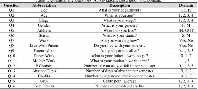
The data set was based on students‟ answers on the preset questionnaire. The questionnaire holds different categories of questions related to students‟ academic performance, their physical activities, residence information, status, work, social activities, and so on. The students were asked to answer 61 questions using a preset questionnaire using LimeSurvey and a Google form questionnaire. LimeSurvey is an open source web application that helped in setting the questionnaire and provided a facility to export results for processing. The questionnaire was set using the network inside the building of the College of Computer Science and Information Technology at the University of Basrah. The total number of participants reached 161 students from two departments (Computer Science Department and Computer Information Systems Department). The data sets from the Google form and LimeSurvey were combined together, and the resulting data set was prepared for the model. Table 1 shows a sample of the questionnaire with abbreviations, question descriptions, and answers domain.
Table 1. Questionnaire Questions, Abbreviations, Description and Domain.
Question Abbreviation Description Domain
Q1 Dep What is your department? CS, IS
Q2 Age What is your age? 1, 2, 3, 4
Q3 Stage What is your stage? 1, 2, 3, 4
Q4 Gender What is your gender? F, M
Q5 Address Where do you live? IN, OUT
Q6 Status What is your status? S, M
Q7 Work Are you working now? Yes, No
Q8 Live With Parent Do you live with your parents? Yes, No
Q9 Parent Alive Are your parents alive? 0, 1, 2, 3
Q10 Father Work What is your father‟s work scope? 0, 1, 2
Q11 Mother Work What is your mother‟s work scope? 1, 2
Q12 F Courses Number of courses you fail in per semester 0, 1, 2, 3
Q13 Absence Days Number of days of absence per semester 0, 1, 2
Q14 Credits Number or registered credits per semester 0, 1, 2
Q15 GPA Grade point average 1, 2, 3, 4
Q17 Years of Study Number of academic years until the present 1, 2, 3, 4, 5 Q18 List Impor Points I can write down the important points while reading the
material.
1, 2, 3, 4, 5
Q19 Write Notes During lectures, I can write notes and use them for exam
preparation.
1, 2, 3, 4, 5
Q20 Prep Study Schedule I prepare a time schedule for studying. 1, 2, 3, 4,
5
Q21 Calm Dur Exam During exams, I stay calm and coherent. 1, 2, 3, 4,
5
Q22 LDeg Not Make Me
Fail
Getting low grades does not make me feel like a failure. 1, 2, 3, 4, 5
Question abbreviations are used in the model
implementation because it is not proper to use
question descriptions in the model. Some students
did not complete the questionnaire due to network
problems resulting in an issue where some fields
did
not
fill
with
answers.
There are
different approaches to handling the problem of
missing values [31]; in our model the missing
values will be removed. There are ten total
uncompleted answers (which will be ignored) and
151 completed answers. The final class used in the
prediction is Grade. The grade is derived from the
question (FCourses) and takes the value F if the
number of failed courses (FCourses) is greater than
or equal to one, and P otherwise. The grade
depends on the final class in the model.
B. Applying FS
The FS approach appeared in 1970 when the
size of databases increased and an urgent need for a
new machine learning method to feature selecting
among many features arose. FS has a range of
definitions, such as “finding the necessary and
sufficient minimum sized set of features to the final
feature” or “finding the best features subset to
improve prediction accuracy or increase the size of
data in order to improve the prediction accuracy”
[32]. FS aims to find the correlated and most
effective attribute, and remove the uncorrelated
features among those of the specific target
attribute. Using FS may increase machine learning
speed and improve the quality of the goal attribute
by selecting only the attributes related to the final
one. FS uses statistical approaches to find
correlation such as Relief, SVM, Info Gain,
Correlation and PC [33, 34]. FS is considered to be
one of the pre-processing steps in DM, and falls
into two categories: wrapper and filter models. The
filter model depends on the characteristics of
training data to find the correlated features without
any learning algorithm, while the wrapper uses a
predefined learning algorithm to determine and
select features based on their performance [35, 36].
Before applying feature selection algorithms, the
final class is determined based on question number
(12), which is the number of failed courses. The
final class (Grade) is set to (F) if the number of
failed courses is greater than 0, and set to (P) if the
number of failed courses is zero. Since there are 61
questions in the dataset, it is necessary to determine
the most correlated questions affecting the final
class and ignore the other questions. Different
studies and models have depended on a specific
algorithm to find the questions most correlated to
the final class. In our model, four algorithms are
tested and give different results. The basic
operation of the feature selection algorithm is to
find the correlation between the final class and
each attribute and give a rank number which
determines the correlation level. Feature selection
is used in different papers related to EDM, such as
[14].
Another model implemented feature selection based on PCA [37]. In our model, four algorithms (Info Gain Attribute Evaluation, Correlation Attribute Evaluation, SVM Attribute Evaluation, and Principal Components) were tested to determine which questions had the most important effect on the final class. The algorithms‟ names were shortened for ease of explanation, as shown in Table 2.Table 2. Feature Selection Algorithms Abbreviations
Algorithm Name Abbreviation
Info Gain Attribute Eval Info Gain
Correlation Attribute Eval Correlation
SVM Attribute Eval SVM
Principal Components PC
a) Info Gain
In this algorithm, attribute evaluation was performed by estimating the information gain according to each class. By using a minimum description-length-based discretization method, numeric attributes were discretized (or binarized). This method treats the missing values by either distributing the counts among
the other values according to their frequency or regarding them as separate values [38]. In Info Gain, the decrease in entropy is measured when the feature is absent. It has been reported that Info Gain achieves its best performance at multi-class benchmarks. For the nominal values, Info Gain takes on a generalized form [33]. Info Gain measured by the decrease of X entropy caused by Y and is represented by:
IG(X|Y) = H(X)-H(X|Y)
Based on this measurement, the Y-feature is more correlated to the X-feature than to the Z-feature if IG(X|Y ) > IG(Z|Y ). IG normalizes the values falling within the range [0,1] where the value 1 indicates that the predicted values is completely correct and value 0 indicates that X is independent of Y. IG treats a pair of features symmetrically. Entropy-based measures can be applied to determine the correlation between nominal and continuous features [35, 39, 40].
b) Correlation
In this method, the correlation is measured based on Pearson‟s correlation between the determined feature and all other features by treating the nominal values as indicators. The overall correlation is produced as a weighted-average rank [38]. Two approaches to estimate the correlation between two features exist. The first measures the correlation using classical linear correlation, while the other uses information theory. The linear correlation coefficient is the measure of the first approach. For two variables (X, Y), the linear correlation coefficient is measured as:
where (x_i) ̅ represents the mean of X, and (y_i) ̅ represents the mean of Y. The value of r falls in the range of [-1,1]. When variables X and Y correlate, r takes the value of 1 to represent the complete correlation between the variables, and takes the value of -1 when a correlation between the variables does not exist [35].
c) Support Vector Machine (SVM)
The SVM is considered one of the effective classification methods, wherein the process of obtaining feature importance is not the main scope. The F-score is a simple approach used to measure the differentiation of two sets of numbers. For a given number of positive and negative instances, which are represented in n+ and n- for a given number of training
vectors xk, k=1, .. n, F(i) represents the F-score of the ith feature is measure as follow:
where X ̅ _i^((+)), X ̅_i^((-)), X ̅_i represent the ith average feature of the positive, negative and whole data sets respectively, X_(k,i)^((+)) and X_(k,i)^((-)) represent the ith feature of the kth positive and negative instances. The discrimination between the positive and negative feature sets is calculated in the numerator, wherein the one within both sets is calculated in the denominator. The feature is assumed to be more discriminative if the F-score is large. Therefore, this score is used as a criterion for feature selection. However, the F-score does not identify the mutual correlation information among features [41].
In general, the SVM arranges the features based on the size of the coefficients. The learning algorithms are repeatedly applied based on the sophisticated variant. The process of identifying the correlated features includes the following two important steps: it attributes the ranking based on the coefficients, and eliminates the low ranked features. These two features are repeated until all the features have been removed. This process of recursive feature elimination has proven its accuracy and has produced better results on specific datasets [38]. An optimal hyper-plane is constructed to separate the set of positive examples with a maximum margin of 1 from negative examples. The SVM proves its accuracy by solving classification problems found in many handwritten recognition cases, face detection, and prediction [42].
d) Principle Component Analysis (PCA)
Principle Component Analysis in Weka is a statistical method used to represent dimensions of data within a low space. One of the primary uses of PCA is feature reduction, wherein the data with a high number of attributes can be represented and visualized in a low number of attributes. For example, data consisting of more than one hundred attributes can be represented by data records with two or three features [43]. The PCA performs data analysis based on multi-valued data analysis, wherein the data table is represented as a data matrix. Aside from attribute reduction, the PCA can be used for data reduction, wherein many data records can be approximated and reduced based on a complex model structure [44].
principle components (PCs) is an important stage in the implementation of the PCA. The determination process for the optimal number of PCs is implemented based on certain criteria. Based on this criteria, the PCs are selected when the cumulative percentage of variance is higher than the threshold value. The practical details of the dataset determine the threshold and often, the threshold falls within the range [70%-90%]. However, an ideal determination of threshold value does not exist; thus, it is heuristically selected. The p number of PCs is chosen when the PCs represent the data in their best form [42].
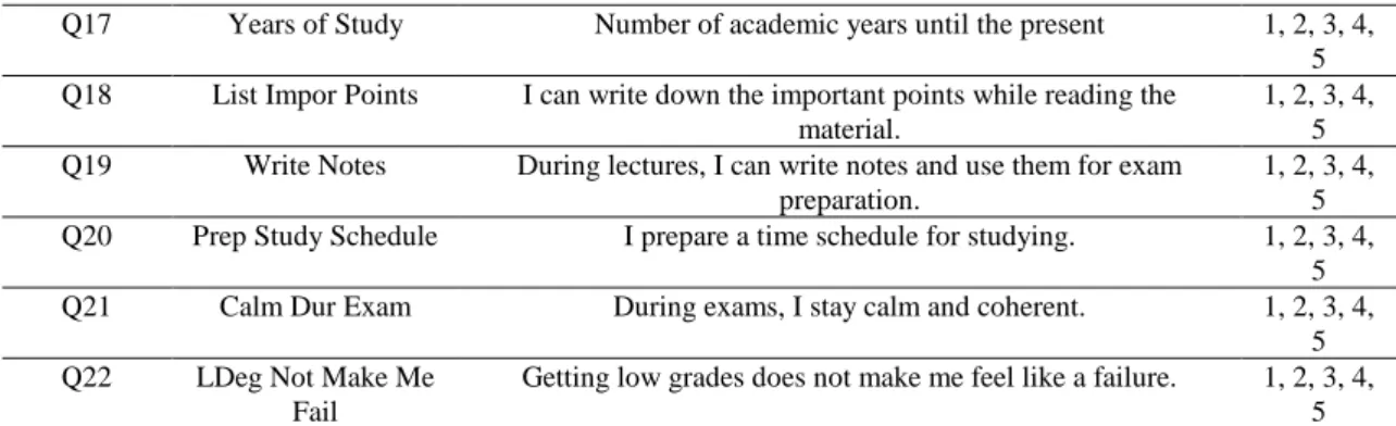
FS algorithms are applied to the data set, and the result ranks of the features are observed. The features in the dataset represent the questions, and the measurement is conducted to identify the affected range between the questions and the final class (Grade). Each FS algorithm produces the correlation as a rank for the features (questions), and measures the correlation between the questions and the final class. Table (3) ranks the questions based on four FS algorithms (Info Gain, Correlation, SVM and PC). The table lists the result in ascending order according to rank, wherein the
algorithms differ in their measurement of the correlation between the questions and the final class. In the table, QN refers to the question number and AVG refers to the average of ranking throughout cross-validation. The question with a rank of one in the information gain algorithm is QN 15 with AVG 0.173, whereas the question with a rank of one in the correlation is QN 15 with AVG 0.451. In the SVM algorithm, QN 26 is the first ranked question with AVG 57.5 and in PC, the QN 61 is the first ranked question. The rest of the table lists the rest of the 59 ranked questions according to the FS algorithms, which are classified by the AVG.
Table 3. Correlation of Attributes According to Feature Selection Algorithms
RANK Info Gain Correlation SVM PC
AVG QN AVG QN AVG QN QN
1 0.173 15 0. 451 15 57.5 26 61 2 0.062 18 0.315 26 57.2 30 19 3 0.055 61 0.233 47 54.7 10 20 4 0.013 8 0.237 16 53.5 58 18 5 0.002 6 0.236 61 53.4 18 22 6 0.002 4 0.235 18 52.3 33 17 7 0.002 5 0.211 48 49.8 41 21 8 0.001 1 0.211 52 49.4 15 23 9 0.051 26 0.186 10 46.5 49 30 10 0 7 0.168 14 42.9 16 27 11 0.037 48 0.17 46 41.7 9 28 12 0.006 16 0.167 30 41.1 45 26 13 0 17 0.163 24 39.7 13 24 14 0.035 47 0.158 36 39 52 25 15 0.033 46 0.156 41 38.9 38 16 16 0 19 0.159 58 38.7 35 15 17 0.005 45 0.153 44 38.4 34 14 18 0 13 0.156 28 37.8 4 4 19 0 21 0.152 17 37.5 27 5 20 0 20 0.144 35 37.3 25 3 21 0 14 0.143 39 36 61 13 22 0 22 0.147 19 33.9 24 2 23 0 11 0.143 59 33.5 5 6 24 0 49 0.135 8 32.8 19 7 25 0 2 0.125 38 32.3 23 8 26 0 3 0.12 60 31.6 28 9 27 0.005 24 0.119 31 30.7 3 12 28 0 23 0.113 54 30.7 43 11 29 0 55 0.107 51 30.6 46 10 30 0 53 0.1 9 29.9 48 29 31 0 59 0.101 53 29.4 51 31 32 0 56 0.094 20 28.2 37 60 33 0 58 0.095 43 27.3 40 50 34 0 57 0.09 50 26.8 42 51
35 0 10 0.085 11 26.4 17 49 36 0 9 0.085 25 26.1 60 53 37 0 50 0.087 27 25.3 8 48 38 0 52 0.078 49 24.9 22 52 39 0 51 0.076 37 24.5 11 54 40 0 25 0.071 21 23.5 2 32 41 0.006 41 0.069 42 23.2 7 58 42 0.009 30 0.064 56 22.4 50 59 43 0 40 0.062 32 20.8 39 57 44 0 42 0.059 23 20.7 59 55 45 0 39 0.051 3 20.4 36 56 46 0 43 0.046 6 20.2 29 47 47 0 45 0.05 45 18.2 47 45 48 0 44 0.049 4 18 57 35 49 0 27 0.042 5 17.3 31 36 50 0 38 0.037 57 17 6 34 51 0 37 0.033 2 16.5 20 44 52 0 28 0.028 13 16.5 32 33 53 0 29 0.028 34 16.3 56 37 54 0 36 0.027 40 15.7 44 38 55 0 60 0.03 1 15.3 53 39 56 0 35 0.028 55 14.3 54 40 57 0 34 0.025 29 12.9 55 43 58 0 33 0.023 33 12 1 42 59 0 32 0.018 7 11.8 21 41 60 0 31 0.018 22 8.8 14 1
Table (3) lists the correlation of attributes according to feature selection algorithms among all the questions. The question 12 FCourses (the number of failed courses) was removed from the dataset since it is replaced by Grade class. Since the final class (Grade) is derived from this question, it assumes the highest correlation to the final class by default. To get better clarification for the table (3), figure (1) lists the
questions and shows the cumulative rank of each question within the FS methods. The rank of each question is represented by a color that determines the method of FS. The figure shows the cumulative rank of all FS methods for each question to identify the less ranked class (highest correlated) to the final class.
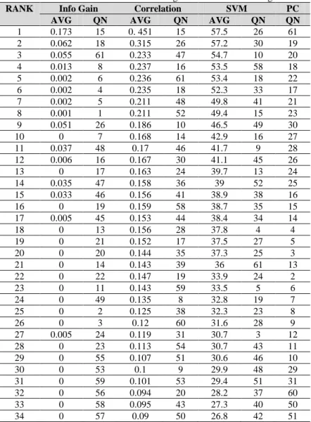
The next step depends on the results found
in table (4), which requires building a table that shows the Average Rank (AVG rank) of each question based on the selected FS algorithms. The new column in the table is calculated based on the following simple equation:After calculating the AVG Rank of each question, the table is sorted in ascending order based on the AVG
Rank to identify the highest correlated questions. The question with lowest AVG Rank is the highest correlated question to the final class because the less rank question in the FS algorithm, the highly correlated to the final class.
Table 4. Average Rank of Correlations In The Algorithms
QN Rank of Info Gain Rank in Correlation Rank in SVM Rank in PC AVG Rank 18 2 6 5 6 4.75 26 9 2 1 14 6.5 15 1 1 8 17 6.75 61 3 5 21 1 7.5 16 12 4 10 16 10.5 19 16 22 24 4 16.5 24 27 13 22 8 17.5 10 35 9 3 29 19 17 13 19 35 15 20.5 30 42 12 2 30 21.5 47 14 7 30 37 22 4 6 48 18 18 22.5 8 4 24 37 25 22.5 48 11 38 9 35 23.25 58 33 16 4 41 23.5 5 7 49 23 19 24.5 51 39 8 14 38 24.75 23 28 44 25 5 25.5 9 36 30 11 26 25.75 20 20 32 51 2 26.25 28 52 18 26 10 26.5 25 40 36 20 13 27.25 13 18 52 13 27 27.5 46 15 3 47 46 27.75 14 21 10 60 21 28 27 49 37 19 12 29.25 3 26 45 27 20 29.5 41 41 15 7 56 29.75 21 19 40 59 3 30.25 6 5 46 50 23 31 11 23 35 39 28 31.25 22 22 60 38 7 31.75 45 17 47 12 51 31.75 50 37 29 31 34 32.75 49 24 34 42 33 33.25 7 10 59 41 24 33.5
45 47 11 29 47 33.5 2 25 51 40 22 34.5 59 31 23 44 42 35 35 56 20 16 50 35.5 38 50 25 15 53 35.75 31 60 27 49 9 36.25 60 55 26 36 32 37.25 53 30 28 56 39 38.25 52 38 31 55 36 40 36 54 14 45 48 40.25 33 58 58 6 40 40.5 39 45 21 43 54 40.75 43 46 33 28 58 41.25 29 53 57 46 11 41.75 37 51 39 32 49 42.75 56 32 42 53 45 43 57 34 50 48 43 43.75 44 48 17 54 57 44 42 44 41 34 59 44.5 34 57 53 17 52 44.75 1 8 55 58 60 45.25 32 59 43 52 31 46.25 40 43 54 33 55 46.25 55 29 56 57 44 46.5
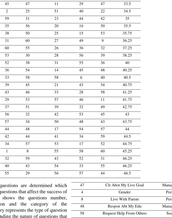
Now the top 30 questions are determined which represent the highest questions that affect the success of students. Table (5) shows the questions number, questions abbreviation and the category of the questions. The category represents the type of question and used for understanding the nature of questions that affect the final class.
Table 5. Top 30 Correlated Questions
QN Question Abbreviation Question
Category
18 List Impor Points Academic
26 Exi To Mater Academic
15 GPA Academic
61 IHv Skills For Self Feel Social
16 Com Credits Academic
19 WriteNotes Academic
24 Eas Can Chos Colg Study Academic
10 Father Work Parent
17 Years Of Study Academic
30 Make Friendship Social
47 Clr Abot My Live Goal Managerial
4 Gender Person
8 Live With Parent Person
48 Respon Abt My Edu Managerial
58 Request Help From Others Social
5 Address Person
51 Clr Idea About Plans Managerial
23 Eas Can Chos Colg Study Academic
9 Parent Alive Parent
20 Prep Study Schedule Academic
28 Dev Relation With Others Social
25 Cn Study Ev UImpo Both Me Academic
13 Absence Days Academic
46 Edu Is LiveJ ob Academic
14 Credits Academic
27 Clr Idea Abt Benifit Managerial
3 Stage Academic
41 Contrl My Budget Managerial
6 Status Person
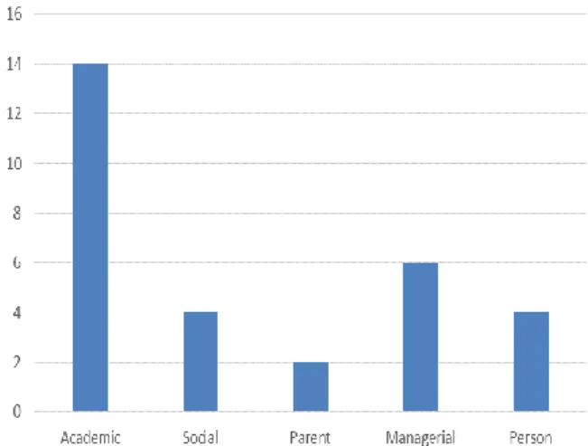
Based on the table (5), figure (2) list the top correlated category of questions that affect the students‟ success. It can be clearly seen that the first category of questions that affect students success is the academic questions followed by a managerial, person, social and finally parent questions. 14 out of 30 questions (academic questions) directly affect the final goal.
Figure 2. Number of Correlated Questions According To Category
C) ANN
The third step in the model is implementing ANN over the dataset after removing the uncorrelated features. ANN is a framework to implement machine learning algorithms on data sets. To get better clarification of ANN framework, the following sections explain ANN parts:
a) Biological & Artificial Neurons
Individual nerve cells or neurons are the basic units of the brain. The human brain contains a huge number of highly connected neurons (approximately 1011 neurons with 104 connections per each), that can be classified into at least a thousand different types [23, 45].
These neurons have three principal components: the dendrites, the cell body, and the axon. The dendrites are tree-like receptive networks of nerve fibers that carry electrical signals into the cell body. The cell body effectively sums and thresholds these incoming signals. The axon is a single long fiber that carries the signal from the cell body out to other neurons [23, 45, 46].
There are two key similarities between biological and artificial neural networks. First, the building blocks of both networks are simple computational devices (although artificial neurons are much simpler than biological neurons) that are highly interconnected. Second, the connections between neurons determine the function of the network [45].
b) Neuron Model
There are two models of neuron [23, 45, 46]:
1- First: Single-Input Neuron
The scalar input p is multiplied by the scalar weight w to form pw, one of the terms that are sent to the summer. The other input, 1, is multiplied by a bias b, and then passed to the summer. The summer output (net input), n, goes into a transfer function, which produces the scalar neuron output, a, as illustrated in Figure 3.
Figure 3. Single-Input Neuron.
The transfer function in Figure 3 may be a linear or a nonlinear function of n. A particular transfer function is chosen to satisfy some specification of the problem that the neuron is attempting to solve.
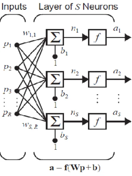
2- Second: Multiple-Input Neuron
Typically, a neuron has more than one input. A neuron with inputs is shown in Figure 4. The individual inputs are each weighted by corresponding elements w1,1, w1,2, w1,3, … w1,R of the weight matrix W.
The neuron has a bias, which is summed with the weighted inputs to form the net input:
This expression can be written in matrix form:
Figure 4. Multiple-Input Neuron.
c) Network Architectures
There are two types of network architectures [23, 45, 46]:
1- First: Single-layer network
In this type of network architecture, each of the inputs R is connected to each of the neurons and that the weight matrix now has S rows.
Figure 5. Single-Layer Network.
Figure (5) shows that each element of the input vector p is connected to each neuron through the weight matrix W. Each neuron has a bias bi, a summer, a transfer function and an output ai. Taken together, the outputs from the output vector a. You can define a single (composite) layer of neurons having different transfer functions by combining two of the networks. Both networks would have the same inputs, and each network would create some of the outputs.
2- Second: Multiple Layers of Neurons
Now consider a network with several layers. Each layer has its own weight matrix W, its own bias vector b, a net input vector n and an output vector a.
If we have three layers of neurons, then the final output is calculated like that:
d) Learning Rules
By learning the rule, we mean a procedure for modifying the weights and biases of a network. The purpose of the learning rule is to train the network to perform some task. They fall into three broad categories: supervised learning, unsupervised learning, and reinforcement (or graded) learning [45-47].
In supervised learning, the learning rule is provided with a set of examples (the training set) of proper network behavior:
where pQ is an input to the network and tQ is the corresponding correct (target) output. As the inputs are applied to the network, the network outputs are compared to the targets. The learning rule is then used to adjust the weights and biases of the network in order to move the network outputs closer to the targets.
Reinforcement learning is similar to supervised learning, except that, instead of being provided with the correct output for each network input, the algorithm is only given a grade. The grade (or score) is a measure of the network performance over some sequence of inputs. In unsupervised learning, the weights and biases are modified in response to network inputs only. There is no target outputs available. Most of these algorithms perform some kind of clustering operation. They learn to categorize the input patterns into a finite number of classes. This is especially useful in such applications as vector quantization [47].There are many uses of ANN, some of them are listed below [48]:
1- Classification
Classification, the assignment of each object to a specific "class", is of fundamental importance in a number of areas angling from image and Speech recognition to the social sciences [49].
2- Clustering
Clustering requires grouping together objects that are similar to each other. In classification problems, the identification of classes known beforehand. In clustering problems, on the other hand, all that is available is a set of samples and distance relationships that can be derived from the sample descriptions.
Vector quantization is the process of dividing up space into several connected regions (called "Voronoi regions"), a task similar to clustering. Each region is represented using a single vector (called a "codebook vector"). Every point in the input space belongs to one of these regions and is mapped to the corresponding (nearest) codebook vector.
Weka tool provides a classifier called (MultilayerPrecepron) to implement NN algorithm. This classifier uses the concept of backpropagation to classify the instances. After dividing data into 70% train data and 30% test data with a specific number of neurons (2 or 3 or 4 or 5 or any number), the result performance criteria of ANN prediction are presented in table (6):
Table 6. ANN Performance Criteria
TP Rate FP Rate Precision Recall
0.871 0.184 0.871 0.871
The performance criteria consist of True positive rate (TP rate) which represents the truly correctly predicted cases and calculated as follow:
where: TP refers to true positives: number of cases
predicted positive that are actually positive and FN refers to false negatives: number of cases predicted negative that are actually positive. The more TP rate, the more accurate predicted answers of students.
False Positive rate (FP rate) represents the incorrectly classified cases and measured as follow:
where FP refers to false positives: the number of cases predicted positive that is actually negative and TN refers to true negatives: a number of cases predicted negative that are actually negative.
Precision represents the positive predicted values (PDV) and used with a recall to measure the relevance and measured as follow:
Recall represents the sensitivity and used with precision to measure the relevance and measured as follow:
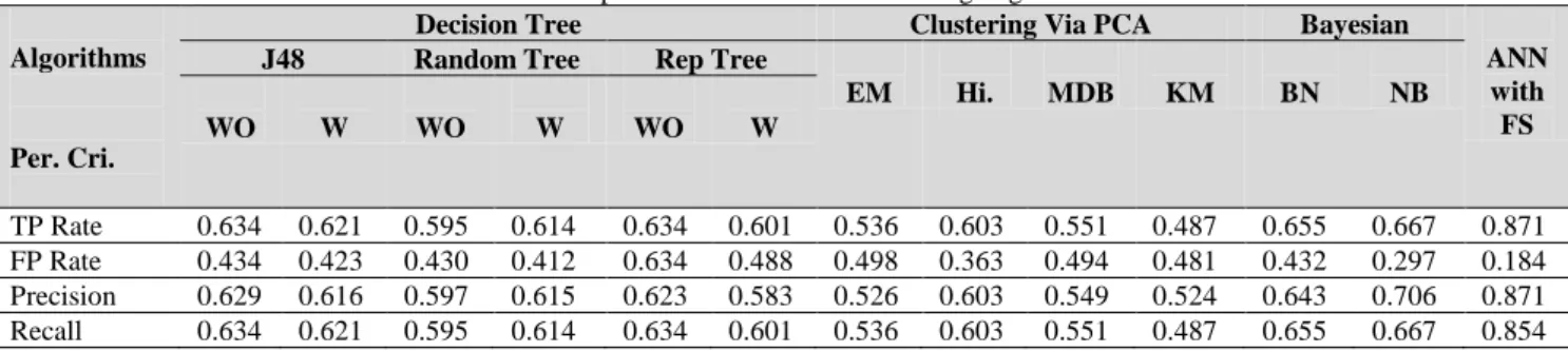
Table 7. Comparison With Other Data Mining Algorithms:
Algorithms
Per. Cri.
Decision Tree Clustering Via PCA Bayesian
ANN with FS
J48 Random Tree Rep Tree
EM Hi. MDB KM BN NB WO W WO W WO W TP Rate 0.634 0.621 0.595 0.614 0.634 0.601 0.536 0.603 0.551 0.487 0.655 0.667 0.871 FP Rate 0.434 0.423 0.430 0.412 0.634 0.488 0.498 0.363 0.494 0.481 0.432 0.297 0.184 Precision 0.629 0.616 0.597 0.615 0.623 0.583 0.526 0.603 0.549 0.524 0.643 0.706 0.871 Recall 0.634 0.621 0.595 0.614 0.634 0.601 0.536 0.603 0.551 0.487 0.655 0.667 0.854
As a comparison between this model and previous models that been implemented on the same data set, the table (7) shows promising accuracy result compared with other data mining techniques. The first model [50] has been implemented using decision tree algorithms (J48 or C4.5, Random Tree and Rep Tree) and with two cases (with attribute filter (W) and without attribute filter (WO)). The highest TP rate and recall (0.634) registered when the classifier (J48 and Rep Tree) applied without attribute filter. These two algorithms also registered the highest precision (0.629 and 0.623), while the lowest FP rate (0.412) registered in Random Tree.
The second model [37] classify the students‟ answers
using four clustering algorithms (EM, hierarchal clustering (Hi), Make Density Based (MDB) and K-Means (KM)). The Hi. algorithm scored the highest performance criteria (TP=0.603, FP=0.363, Precision=0.603 and Recall=0.603).
The third model [9] implemented the prediction model based on two Bayes algorithms (Bayes Network (BN) and Naïve Bayes (NB)). The NB algorithm scored the highest performance criteria (TP=0.667, FP=0.297, Precision=0.706 and Recall=0.667).
Based on the criteria of these three models, the performance criteria of ANN with Feature Selection (FS) scored the high measurements compared with these three models. ANN with FS scored (TP=0.871, FP=0.184, Precision=0.871 and Recall=0.854). Based
on these performance criteria, this model can be considered as an optimal model compared with the
previous models.
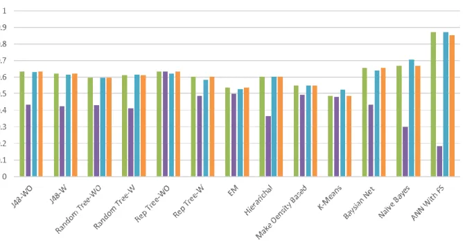
Figure 6. Models Performance
Figure (6) is demonstrated based on the table (7) to give a better view for the performance criteria of the four models. It can be clearly seen that ANN with FS as a comparison with the three previous models predicts the final goal with high accuracy rate, precision and recall, and low FP rate.
The next step is listing the prediction margin of predicted answers. Prediction margin can measure the accuracy of prediction of each single predicted answer. This margin can prove and support the accuracy of model performance.
Figure 7. Prediction Margin
Figure (7) demonstrates the actual values of the test set of the data set and the predicted value of each answer with prediction margin. The prediction margin is a value that falls in a range between -1 and 1. Prediction margin is the difference result of predicted probability between the highest predicted and the actual class. The highest prediction margin, the more accurate
classifier prediction which means when the prediction margin reaches 1, the prediction result of the class is highly accurate. When the prediction margin reaches to -1, the prediction result of class is incorrect. Since the prediction precision is 87%, so there are incorrect predicted values which reach 13% of the overall predicted cases. The prediction margin reached to 1 (100% correct) for 25 out of 28 correctly predicted cases where the remaining 3 predicted cases reached to average 0.8.
IV. C
ONCLUSIONSIn this paper, a proposed EDM model based on ANN and a combination of FS methods are presented. The proposed model can predict the academic performance of the students in the university based on their answers on specific questions. The model implemented by collecting students‟ answers in a questionnaire. This questionnaire consists of two parts, the first part designed in LimeSurvey application and the second one designed by online Google form. The questionnaire consists of 61 questions and these question varied such as social activities, sport, academic activity, parent jobs, and managerial activity. Since it is not prudent to take all the questions into consideration because there are many uncorrelated questions that may affect the model accuracy, so there is a need for questions elimination. One of the FS tasks is finding the correlation among attributes in order to remove the
features with less correlation and keep only the highest correlated features.
FS methods vary in their approaches to finding the correlation among features. Since this variation may produce different ranks of correlation for features for a single data set, so four selected FS method is used in this model to compare their performances and take the average rank. The top 30 questions classified into categories which group the field topic of the question such as (academic, parent, person, managerial and social). Based on implementing four FS algorithms, it been concluded that academic factors affect the success of students. 14 academic factors out of the first 30 factors influenced the final factor (Grade). The next factor categories that affect the success are managerial 6 factors, social and person 4 factors and parent 2 factors sequentially. ANN is used in many fields and for many machine learning functions and proved its accuracy in these fields. ANN with FS is used in the field of students‟ success prediction in the model.
After dividing the data set into 70% for training the model and 30% for testing data, the model is tested the test data and give the predicted answers with accuracy reached to 87% with any number of neurons greater than 1. A comparison is made between the model and three previous models in the field of students‟ success prediction and showed that ANN with FS model scored the highest accuracy in the performance criteria (TP rate, precision, and recall) with the lowest score in FP rate. A prediction margin for predicted answers is presented to prove the accuracy of the prediction mode. The prediction margin reached to 1 (100% correct) for 25 out of 28 correctly predicted cases where the remaining 3 predicted cases reached to average 0.8.
Although it is important for academic staff to find the factors that enhance academic performance and that is what FS gives, but it very important to them to find how these factors affect and improve academic performance. Since FS methods give the features‟ ranks that represent the correlation between the features and the final feature so the next step is finding how these features (questions) can increase the success and reduce students‟ failure by measure the feature influence on the final class alone.
A
CKNOWLEDGMENTSI „d like to express my deep appreciation to the staff of the deanery of College of Computer Science and Information Technology for their help and cooperation. I also appreciate the help provided by my colleagues Assist. Lecturer Ali Salah Hashim and Assist. Lecturer Wid Akeel Awadh for their help in implementing the questionnaire. My special thanks to all students that participated in the questionnaire and gave their time to
answer all the questions.
R
EFERENCES[1]
T. BARNES and J. STAMPER. (2007)
"Toward the extraction of production rules
for solving logic proofs," in AIED07, 13th
International Conference on Artificial
Intelligence in Education, Educational Data
Mining Workshop, pp. 11-20.
[2]
R. S. BAKER and P. S. INVENTADO,
"Educational data mining and learning
analytics," in Learning analytics, ed:
Springer, 2014, pp. 61-75.
[3]
S. K. MOHAMAD and Z. TASIR. (2013)
"Educational data mining: A review,"
Procedia-Social and Behavioral Sciences,
97, pp. 320-324.
[4]
B. K. BARADWAJ and S. PAL. (2012)
"Mining educational data to analyze
students' performance," arXiv preprint
arXiv:1201.3417,.
[5]
A. K. HAMOUD. (2016) "Selection of Best
Decision Tree Algorithm for Prediction and
Classification of Students‟ Action,".
[6]
Z. KOVACIC. (2010) "Early prediction of
student
success:
Mining
students'
enrolment data".
[7]
M.
RAMASWAMI
and
R.
RATHINASABAPATHY. (2012) "Student
Performance
Prediction,"
International
Journal of Computational Intelligence and
Informatics, 1.
[8]
M. XENOS. (2004) "Prediction and
assessment of student behaviour in open
and distance education in computers using
Bayesian
networks,"
Computers
&
Education, 43, pp. 345-359.
[9]
A. HAMOUD, A. HUMADI, W. A.
AWADH, and A. S. HASHIM. (2017)
"Students‟ Success Prediction based on
Bayes Algorithms".
[10]
A. M. HUMADI and A. K. HAMOUD.
(2017) "Online Real Time Fuzzy Inference
System Based Human Health Monitoring
and Medical Decision Making"
[11]
O. TAYLAN and B. KARAGÖZOĞLU,
(2009) "An adaptive neuro-fuzzy model for
prediction
of
student‟s
academic
performance," Computers & Industrial
Engineering, vol. 57, pp. 732-741,.
[12]
S. T. KARAMOUZIS and A. VRETTOS
(2008) "An artificial neural network for
predicting student graduation outcomes,"
in Proceedings of the World Congress on
Engineering and Computer Science, pp.
991-994.
[13]
B. C. HARDGRAVE, R. L. WILSON, and
K. A. WALSTROM (1994) "Predicting
graduate student success: A comparison of
neural
networks
and
traditional
techniques," Computers & Operations
Research, 21, pp. 249-263.
[14]
A. S. HASHIMA, A. K. HAMOUD, and
W. A. AWADH. (2018) "Analyzing
students’ answers using association rule
mining based on feature selection," Journal
of Southwest Jiaotong University, 53.
[15]A. JAIN and D. ZONGKER. (1997)
"Feature selection: Evaluation, application,
and small sample performance," IEEE
transactions on pattern analysis and
machine intelligence, 19, pp. 153-158.
[16]
M.
RAMASWAMI
and
R.
BHASKARAN, (2009) "A study on feature
selection techniques in educational data
mining," arXiv preprint arXiv:0912.3924.
[17]M.
ALABBAS,
S.
JAF,
and
S.
KHUDEYER. (2018) "Combining machine
learning classifiers for the task of arabic
characters recognition," The international
journal of Asian language processing
(IJALP), 28, pp. 1-12.
[18]
M. ALABBAS, R. S. KHUDEYER, and S.
JAF. (2016) "Improved Arabic characters
recognition by combining multiple machine
learning classifiers," in Asian Language
Processing (IALP), 2016 International
Conference on, pp. 262-265.
[19]
M. M. KHUDHAIR and A. H. H.
ALASADI. (2011) "Applying New Method
for Computing Initial Centers of K-means
clustering
with
Color
Image
Segmentation," JOURNAL OF THI-QAR
SCIENCE, 3, pp. 116-124.
[20]
A. H. H. ALASADI, H. MOHAMMED,
and E. N. ALSHEMMARY. (2013)
"Hybrid k-means Clustering for Color
Image
Segmentation,"
Science
and
Engineering (IJCSE), vol. 2, pp. 17-26.,.
[21]
A. H. KHALEEL. (2016) "An efficient
approach for medical text categorization
based
on
clustering
and
similarity
measures," Misan Journal of Acodemic
Studies, 15, pp. 113-131.
[22]
M. PALIWAL and U. A. KUMAR. (2009)
"Neural
networks
and
statistical
techniques: A review of applications,"
Expert systems with applications, 36, pp.
2-17.
[23]
E. R. KANDEL, J. H. SCHWARTZ, T. M.
JESSELL, D. o. BIOCHEMISTRY, M. B.
T. JESSELL, S. SIEGELBAUM, et al.
(2000) Principles of neural science, 4:
McGraw-hill New York.
[24]
M. A. ULKAREEM, W. A. AWADH, and
A. S. ALASADY. (2018) "A comparative
study to obtain an adequate model in
prediction of electricity requirements for a
given future period," in 2018 International
Conference on Engineering Technology
and their Applications (IICETA), pp.
30-35.
[25]
A. Y. ABDALLA, T. Y. ABDALLA, and
K. A. NASAR. (2012) "Routing with
Congestion Control in Computer Network
using Neural Networks," International
Journal of Computer Applications, 57.
[26]A. A. KARDAN, H. SADEGHI, S. S.
GHIDARY, and M. R. F. SANI (2013),
"Prediction of student course selection in
online higher education institutes using
neural network," Computers & Education,
65, pp. 1-11.
[27]
S. BORKAR and K. RAJESWARI. (2013)
"Predicting students academic performance
using education data mining," International
Journal of Computer Science and Mobile
Computing, 2, pp. 273-279,.
[28]
A. CRIPPS. (1996) "Using artificial
neural
nets
to
predict
academic
performance," in Proceedings of the 1996
ACM symposium on Applied Computing, ,
pp. 33-37.
ECONOMIDES. (2009) "Prediction of
student‟s mood during an online test using
formula-based and neural network-based
method," Computers & Education, 53, pp.
644-652.
[30]
V. OLADOKUN, A. ADEBANJO, and O.
CHARLES-OWABA. (2008) "Predicting
students‟ academic performance using
artificial neural network: A case study of an
engineering course," The Pacific Journal of
Science and Technology, 9, pp. 72-79.
[31]B. M. HUSSAN, G. a.-S. KHALEEL, and
A. HAMEED (2012) "Studying the Impact
of Handling the Missing Values on the
Dataset On the Efficiency of Data Mining
Techniques," Basrah journal of science, 30,
pp. 128-141.
[32]
M. DASH and H. LIU. (1997) "Feature
selection for classification," Intelligent data
analysis, 1, pp. 131-156.
[33]
G. FORMAN. (2003) "An extensive
empirical study of feature selection metrics
for text classification," Journal of machine
learning research, 3, pp. 1289-1305.
[34]
K. KIRA and L. A. RENDELL. (1992) "A
practical approach to feature selection" in
Machine Learning Proceedings ed:
Elsevier, pp. 249-256.
[35]
L. YU and H. LIU. (2003) "Feature
selection for high-dimensional data: A fast
correlation-based
filter
solution,"
in
Proceedings of the 20th international
conference
on
machine
learning
(ICML-03), pp. 856-863.
[36]
M. A. HALL (2000) "Correlation-based
feature selection of discrete and numeric
class machine learning".
[37]
A.
K.
HAMOUD.
(2018)
"CLASSIFYING STUDENTS'ANSWERS
USING CLUSTERING ALGORITHMS
BASED ON PRINCIPLE COMPONENT
ANALYSIS," Journal of Theoretical &
Applied Information Technology, 96.
[38]
I. H. WITTEN, E. FRANK, M. A. HALL,
and C. J. PAL. (2016) Data Mining:
Practical machine learning tools and
techniques: Morgan Kaufmann.
[39]
U. FAYYAD and K. IRANI. (1993)
"Multi-interval
discretization
of
continuous-valued
attributes
for
classification learning".
[40]
H. LIU, F. HUSSAIN, C. L. TAN, and M.
DASH,
(2002)
"Discretization:
An
enabling technique," Data mining and
knowledge discovery, 6, pp. 393-423.
[41]
Y.-W. CHEN and C.-J. LIN (2006)
"Combining SVMs with various feature
selection strategies," in Feature extraction,
ed: Springer, pp. 315-324.
[42]
H. TAIRA and M. HARUNO. (1999)
"Feature
selection
in
SVM
text
categorization,"
in
AAAI/IAAI,
pp.
480-486.
[43]
N. YE, (2013) Data mining: theories,
algorithms, and examples: CRC press.
[44]
S. Wold, K. Esbensen, and P. Geladi
(1987) "Principal component analysis,"
Chemometrics and intelligent laboratory
systems, 2, pp. 37-52.
[45]
M. T. HAGAN, H. B. DEMUTH, M. H.
BEALE, and O. De JESÚS (1996) Neural
network design, 20.
[46]
L. V. FAUSETT. (1994) Fundamentals of
neural networks: architectures, algorithms,
and
applications
3:
Prentice-Hall
Englewood Cliffs.
[47]
T.
D.
Sanger.
(1989)
"Optimal
unsupervised learning in a single-layer
linear feedforward neural network," Neural
networks, 2, pp. 459-473.
[48]
K. MEHROTRA, C. K. MOHAN, and S.
RANKA (1997), "Elements of Artificial
Neural Networks (Complex Adaptive
Systems)," ed: Cambridge, MA: MIT Press.
[49]
G. HEPNER, T. LOGAN, N. RITTER,
and N. Bryant. (1990) "Artificial neural
network classification using a minimal
training set- Comparison to conventional
supervised
classification,"
Photogrammetric Engineering and Remote
Sensing, 56, pp. 469-473.
[50]
Hamoud, Alaa Khalaf, Ali Salah Hashim,
and Wid Aqeel Awadh. "Predicting Student
Performance
in
Higher
Education
Institutions Using Decision Tree Analysis."
International
Journal
of
Interactive
Multimedia & Artificial Intelligence 5, no.
2 (2018).
参考文:
[1]T. BARNES 和 J. STAMPER。 (2007)
“提取解决逻辑证据的生产规则”,载
于AIED07,第13届教育人工智能国际
会议,教育数据挖掘研讨会,第11-20
页.
[2]R. S. BAKER 和 P. S. INVENTADO,“
教 育 数 据 挖 掘 和 学 习 分 析 ” , 在
Learning analytics,ed:Springer,2014,
pp.61-75.
[3]S. K. MOHAMAD 和 Z. TASIR(2013)
“教育数据挖掘:评论”,“程序 - 社
会和行为科学”,97,第320-324页.
[4]B. K. BARADWAJ和S. PAL. (2012) “挖
掘教育数据以分析学生的表现”,arXiv
preprint arXiv:1201.3417 .
[5]A. K. HAMOUD(2016)“用于预测和
分类学生行为的最佳决策树算法的选择
[6]Z. KOVACIC(2010)“学生成功的早期
预测:挖掘学生的入学数据”.
[7]M.
RAMASWAMI
和
R.
RATHINASABAPATHY(2012)“学生
表现预测”,国际计算智能与信息学杂
志,1.
[8]M. XENOS,(2004)“使用贝叶斯网络
对计算机开放和远程教育中学生行为的
预测和评估”,计算机与教育,43,第
345-359页.
[9]
A. HAMOUD , A 。 HUMADI , W.A.
AWADH和A. S. HASHIM(2017)“基
于贝叶斯算法的学生成功预测”.
[10]A. M. HUMADI 和 A. K. HAMOUD
(2017) “基于在线实时模糊推理系统的
人体健康监测和医疗决策”.
[11]O. TAYLAN 和 B.KARAGÖZOĞLU.
(2009) “用于预测学生学习成绩的自适
应神经模糊模型”,计算机与工业工程
,第一卷 57,pp.732-741.
[12]S. T. KARAMOUZIS 和 A. VRETTOS
(2008)“用于预测学生毕业成果的人工
神经网络”,载于“世界工程与计算机
科学大会论文集”,第991-994页.
[13]B. C. HARDGRAVE,R.L. WILSON和
K. A. WALSTROM(1994)“预测研究
生成功:神经网络与传统技术的比较”
,计算机与运筹学,21,第249-263页.
[14]A. S. Hashima,A. K. Hamoud和W. A.
Awadh,(2018) “使用基于特征选择的
关联规则挖掘来分析学生的答案”,“
西南交通大学学报”,53.
[15]A. JAIN和D. ZONGKER,(1997) “特
征选择:评估,应用和小样本性能”,
IEEE关于模式分析和机器智能的交易,
19,pp.153-158.
[16]M. RAMASWAMI 和 R. BHASKARAN
,(2009)“关于教育数据挖掘中特征
选择技术的研究”,arXiv preprint arXiv
:0912.3924.
[17]M. ALABBAS , S 。 JAF 和 S.
KHUDEYER。 (2018)“结合机器学习
分类器,用于阿拉伯字符识别任务”,
国际亚洲语言处理杂志(IJALP),28, 第
1-12页.
[18]M. ALABBAS,R.S. KHUDEYER和S.
JAF (2016)“通过结合多个机器学习
分类器改进阿拉伯字符识别”,在亚洲
语言处理(IALP),2016年国际会议上
,第262-265页.
[19]M. M. KHUDHAIR和A. H. H. ALASADI
(2011)“应用新方法计算具有彩色图
像分割的K均值聚类的初始中心”,“
THI-QAR SCIENCE” , 第 3 期 , 第
116-124页.
[20]A. H. H. ALASADI,H. MOHAMMED
和E. N. ALSHEMMARY。 (2013)“用
于彩色图像分割的混合k均值聚类”,
“科学与工程”(IJCSE),第一卷。 2
,pp.17-26.
[21]A. H. KHALEEL. (2016)“基于聚类
和相似性度量的医学文本分类的有效方
法 ” , Misan Journal of Acodemic
Studies, 15,pp.113-131.
神经网络和统计技术:应用评论”,应
用专家系统,36,第2-17页.
[23]
E. R. KANDEL,J。H. SCHWARTZ,
TM. JESSELL,D. o。 BIOCHEMISTRY
M.B. T. JESSELL,S。SIEGELBAUM,
et al. ( 2000 ) 神 经 科 学 原 理 , 4 :
McGraw-hill纽约.
[24]M. A. ULKAREEM,W.A. AWADH和
A. S. ALASADY. (2018)“2018 年工程
技术及其应用国际会议(IICETA),第
30-35页,”在预测特定未来时期的电
力需求预测中获得适当模型的比较研究
[25]A. Y. ABDALLA,T.Y. ABDALLA和K.
A. NASAR (2012)“使用神经网络在
计算机网络中进行拥塞控制的路由”,
国际计算机应用杂志,57.
[26]A. A. KARDAN,H。SADEGHI,S。
S. GHIDARY和M. R. F. SANI(2013),
“使用神经网络预测在线高等教育机构
的学生课程选择”,计算机与教育,65
,第1-11页.
[27]S. BORKAR和K. RAJESWARI (2013)“
使用教育数据挖掘预测学生的学业成绩
”,国际计算机科学与移动计算杂志,
2,第273-279页.
[28]A. CRIPPS。 (1996)“使用人工神经
网预测学业成绩”,参见1996年ACM应
用计算研讨会论文集,第33-37页.
[29]C. N. MORIDIS和A. A. ECONOMIDES
。 (2009)“使用基于公式和基于神经
网络的方法在线测试期间预测学生的情
绪 , ” Computers & Education , 53 ,
pp.644-652.
[30]V. OLADOKUN,A。ADEBANJO和O.
CHARLES-OWABA。 (2008)“使用
人工神经网络预测学生的学业成绩:工
程课程的案例研究”,“太平洋科学与
技术杂志”,9,第72-79页.
[31]
B. M. HUSSAN,G. a.-S. KHALEEL和
A. HAMEED(2012)“研究处理缺失值
对数据集对数据挖掘技术效率的影响”
,巴士拉科学杂志,30,第 128-141 页
[32]M. DASH和H. LIU。 (1997)“用于分
类的特征选择”,智能数据分析,1,
第131-156页.
[33]G. FORMAN. (2003)“对文本分类的
特征选择度量的广泛实证研究”,机器
学习研究杂志,3,页1289-1305.
[34]K. KIRA和L. A. RENDELL。 (1992)
“机器学习论文集”中的“一种实用的
特 征 选 择 方 法 ” , 载 : Elsevier , 第
249-256页.
[35]L. YU和H. LIU。 (2003)“高维数据
的特征选择:基于快速相关的滤波器解
决方案”,参见第20届机器学习国际会
议论文集(ICML-03),第856-863页。
[36]M. A. HALL(2000)“离散和数字类机
器学习的基于相关的特征选择”.
[37]A. K. HAMOUD。 (2018)“基于原理
组件分析的分组算法对学生进行分类”
,“理论与应用信息技术期刊”,96。
[38]
I. H. WITTEN , E 。 FRANK, M 。A.
HALL和C. J. PAL。 (2016)数据挖掘
实用的机器学习工具和技术:Morgan
Kaufmann.
[39]U. FAYYAD和K. IRANI (1993)“用
于分类学习的连续值属性的多区间离散
化”.
[40]H. LIU,F。HUSSAIN,C.L。TAN和
M. DASH,(2002)“Discretization:
An enabled technique,”Data mining and
knowledge discovery,6,pp.393-423.
[41]Y.-W.陈和C.-J. LIN(2006)“将SVM
与各种特征选择策略相结合”,在特征
提取中编辑:Springer,第315-324页。
[42]H. TAIRA和M. HARUNO。 (1999)
“AAM / IAAI中的特征选择SVM文本分
类”,第 480-486 页.
[43]N. YE,(2013)数据挖掘:理论,算
法和例子:CRC出版社.
[44]
S. Wold , K 。 Esbensen 和 P. Geladi
(1987) “ Principal component analysis ,
”Chemometrics and intelligent laboratory
systems,2,pp.37-52.
[45]M. T. HAGAN , H 。 B. DEMUTH ,
MH. BEALE和O.DeJESÚS(1996)神经
网络设计,20.
[46]L. V. FAUSETT. (1994)神经网络基础
: 架 构 , 算 法 和 应 用 3 : Prentice-Hall
Englewood Cliffs.
[47]
T. D. Sanger。 (1989)“在单层线性前
馈神经网络中的最优无监督学习”,神
经网络,2,第459-473页.
[48]K. MEHROTRA , C.K. MOHAN 和 S.
RANKA(1997),“人工神经网络的元
素(复杂自适应系统)”,编辑:剑桥
,麻省:麻省理工学院出版社.
[49]G. HEPNER,T. LOGAN,N。RITTER
和N. Bryant (1990)“使用最小训练集
的人工神经网络分类 - 与传统监督分类
的比较”,摄影测量工程和遥感,56,
第469-473页.
[50]