Chapter 1 Market Access and Intermediate Goods
Trade
権利
Copyrights 日本貿易振興機構(ジェトロ)アジア
経済研究所 / Institute of Developing
Economies, Japan External Trade Organization
(IDE-JETRO) http://www.ide.go.jp
journal or
publication title
New Challenges in New Economic Geography
page range
9-42
year
2010-03
9
Kumagai, Satoru ed. 2010. New Challenges in New Economic Geography. Chiba: Institute of Developing Economies.
Chapter 1 Market Access and Intermediate Goods Trade
Kazunobu HAYAKAWA
†§Abstract
This paper examines a distinctive feature of intermediate goods trade which the traditional gravity equation fails to capture, i.e., intermediate goods trade is positively related not only to the importing country‟s demand for finished goods but also to its neighbors‟ demand for finished goods. We regress a gravity equation for finished goods trade in the first step. Then, introducing the importing country‟s access to the total demand for finished goods which is calculated by using the estimates in the first step, we regress our gravity equation for trade in intermediate goods. Our regression results confirm such a feature of intermediate goods trade. Using the results of the regression, we simulate how the rise of US consumers‟ demand for finished goods affects the total imports and exports of intermediate goods in each country.
Keywords: Gravity, intermediate goods trade, OECD JEL Classification: F12, F14, R12
†
Researcher, Economic Integration Studies Group, Inter-Disciplinary Studies Center, Institute of Developing Economies ([email protected])
§
I am grateful to Hiroyuki Kasahara, Kiyoyasu Tanaka, Nobuaki Yamashita, and seminar participants at the Institute of Developing Economies and Keio University.
10
1. Introduction
Given the rapid growth of intermediate goods trade, it is increasingly important to clarify the mechanics of such trade. Worldwide trade in machinery parts and components grew from $336 billion in 1987 to $1,299 billion in 2003, while total commodity trade and trade in machinery goods increased from $2,127 billion to $6,526 billion and from $837 billion to $2,913 billion, respectively (Kimura et al. 2007). As a result, the share of machinery parts and components in total commodity trade and in machinery goods trade increased from 16% to 20% and from 40% to 45%, respectively. In spite of such rapid growth in intermediate goods trade, studies in international economics have primarily investigated the mechanics of trade in consumption goods, i.e., finished goods. It has now become important to pay a special attention to intermediate goods trade.
In international economics, it is well known that a gravity equation is one of the most successful tools for quantitatively analyzing bilateral trade patterns. The traditional gravity equation has a log of bilateral trade as a dependent variable as well as logs of importer‟s and exporter‟s GDPs and a log of distance between trading partners as independent variables. Its estimation always presents us with an excellent empirical fit. Relying on such properties, a large number of scholars have employed a gravity equation for the investigation of bilateral trade. It can be used for clarifying the causes of growth of world trade after the Second World War (Baier and Bergstrand 2001). The impact of international agreements (Baier and Bergstrand 2007), e.g., free trade agreements (FTAs), and international organizations (Rose 2004), e.g., the World Trade Organization, on trade can also be evaluated by the gravity equation. The
11
development of these gravity papers proves the equation‟s usefulness in empirical analysis. In addition, there are now a variety of the theoretical models supporting the gravity formulation (see, for example, Combes et al. 2008: 127). In short, a gravity equation is a powerful tool from both the theoretical and empirical points of view.
However, the traditional gravity equation fails to capture the distinctive features of intermediate goods trade. Basically, if we simply apply the traditional gravity equation to intermediate goods trade, the coefficient for the importer‟s GDP will capture only the role of the importing country‟s demand for finished goods in
intermediate goods trade.1 However, the producers of finished goods in the importing
country do not necessarily import intermediate goods to supply their assembled products only to consumers in the importing country. For example, imports of intermediate goods in Mexico seem to be aimed toward export of the assembled finished goods to the US. Also, Eastern European countries may import intermediate goods from Japan in order to export finished goods to Western European countries. As a result, imports of intermediate goods might be sensitive not only to the magnitude of the importing country‟s demand for finished goods but also to that of its neighboring countries‟ demand. Since the traditional gravity equation includes only the importing country‟s demand for finished goods (i.e., importer‟s GDP), it has remained unknown whether its neighboring countries‟ demand for finished goods is also important for intermediate goods trade or not.
Against this backdrop, we examine the role not only of the importing country‟s
1
Some papers applied the gravity equation basically in the traditional way, only for intermediate goods trade (see, for example, Athukorala and Yamashita 2006, Kimura et al. 2007). Such papers found that gravity works also in intermediate goods trade to some extent; the high importer‟s and exporter‟s GDPs encourage their active intermediate goods trade, while the long distance between them discourages it.
12
demand for finished goods but also of its neighbors‟ demand for finished goods in intermediate goods trade by estimating the modified gravity equation. Our gravity equation is derived from the new economic geography (NEG) model, of which a pioneer work is Krugman (1991). In terms of incorporating regional interaction explicitly, the NEG model is suitable for our purpose. From the NEG model with upstream and downstream sectors, we derive gravity equations for trade in upstream products and downstream products separately. The final goal of this paper is to estimate the gravity equation for trade in upstream products. This includes the importing country‟s demand for upstream products, which depends not only on its demand for downstream products but also on its neighbors‟ demand for downstream products adjusted by trade costs. This importing country‟s access to “the total demand for downstream products” is obtained by using the Redding and Venables (2004) method. In short, we regress a gravity equation for trade in downstream products and obtain the estimates of importer-fixed effects and of some parameters in trade costs function. Using these estimates, we construct each country‟s access to the total demand for downstream products, which is regressed on bilateral trade in upstream products.
This paper contributes not only to the gravity literature but also to the NEG empirics. In the gravity literature, on the one hand, this is the first paper that carefully explores the above-mentioned nature of intermediate goods trade. There are some papers analyzing intermediate goods trade by estimating gravity(-like) equations. For example, Egger and Egger (2005), Athukorala and Yamashita (2006), and Kimura et al. (2007) examine the role of trading partners‟ GDP, their income similarity, and so on. Hayakawa and Kimura (2009) investigate the impact of exchange rate volatility on intermediate goods trade. To the best of our knowledge, no papers have ever examined
13
the role of the importing country‟s access to the total demand for finished goods in intermediate goods trade. However, such an analysis is invaluable because it enables us to investigate the impact of the rise of national income in a country on intermediate goods trade in the world. The importance of this analysis lies in the fact that the national income in a country has no direct relationship with intermediate goods trade in other countries. The indirect path described by our model is as follows: the rise of total income in a country increases the exports of finished goods from the world to that country. Thus, the worldwide expansion of finished goods production leads to a dramatic increase of intermediate goods trade in the world. To visualize such an indirect path to some extent, we simulate how the rise of US consumers‟ demand for finished goods affects the total imports and exports of intermediate goods in each country. The simulation shows that, in spite of the expansion of US demand for finished goods, increases of imports and exports in intermediate goods can be observed in all countries.
In the NEG empirics, on the other hand, our paper extends the application range of the Redding and Venables method. In the NEG model, in general, price index is one of the key variables, but it is troublesome to obtain data for it or control its effects. To tackle this difficulty, the two-step approach proposed by Redding and Venables has been adopted in the literature.2 The estimates in the gravity equation in the first step are used for constructing a market access measure, which takes the price index into account. Then, in the second step, its relationship with other economic variables is examined. Redding and Venables (2004) and some sequential papers (Bosker and Garretsen 2008, Brakman, Garretsen and Schramm 2006, Head and Mayer 2006,
2
14
Hering and Poncet 2009, Knaap 2006, Redding and Schott 2003) used such an approach to examine the relationship between wages and market access. Kheder and Zugravu (2008), Head and Mayer (2004), and Mayer, Mejean and Nefussi (2007) used this approach in the context of a location choice analysis. In this paper, we examine the relationship between intermediate goods trade and market access, and the market access is constructed by using the estimates of a gravity equation for finished goods trade.
The remainder of this paper is organized as follows. The next section provides the theoretical framework underlying our gravity equations. The empirical strategy for estimation of the equations is explained in Section 3, and the regression results are reported in Section 4. Finally, Section 5 presents our conclusion.
2. Theoretical Framework
In this section, we provide our theoretical framework for the empirical analysis. The model is basically similar to Amiti (2005). A representative consumer in each region is assumed to have a two-tier utility function. The upper tier is a Cobb-Douglas function of the utility derived from consumption of downstream goods (finished goods). Specifically, the following utility function of the consumer in country r is applied:
i i r r i C U ,
1 ii ,where Cri is the aggregate consumption of a downstream good i in country r.
Consider expenditure allocation in a downstream good i consisting of multiple varieties differentiated by country (the Armington assumption) with the subscript representing the name of downstream goods omitted for now. A consumer has the
15
following preference specified as a constant elasticity of substitution (CES) function over varieties: 1 1 1
R s sr r X C ,where R and Xsr are the number of countries and the demand of country r for the
downstream variety produced in country s, respectively. σ is the elasticity of substitution between downstream varieties and is assumed to be greater than unity. The utility maximization yields:
r r s sr sr p P Y X (1) 1 , (1)
where ps and Pr denote, respectively, the price of the downstream variety produced in
country s and the price index of downstream goods in country r. Yr is total
expenditure/income in country r. Transactions in downstream goods between countries r and s may be modeled as facing Samuelsonian iceberg costs, τsr (≥1). As a result, the
total production value of downstream industry in country i, which is denoted by Ei (≡
pi Xi), is given by:
i r ir r r i p P Y E ( 1) ( 1) 1 , (2) The market structure in the downstream goods sector is assumed to be perfect competition. The downstream goods producer of each country combines a composite index aggregated across varieties of intermediate inputs and primary factors such as skilled and unskilled labor using a Cobb-Douglas model. This index enters the cost function for each producer through a CES aggregator. Specifically, the following cost function emerges:16
Xr wr Gr Xr C 1 ,
1 1 1 0 ) 1 ( ) 1 (
R s M s sr r t q j dj G s ,where wr denotes the price index for primary factors employed in country r to produce
downstream output Xr (called simply wages). Gr is the price index for upstream
products, and μ is a linkage parameter between downstream and upstream goods. Unlike downstream goods, upstream products are differentiated by firm. Their market structure is assumed to be monopolistic competition. Transactions between countries r
and s in upstream products are modeled as facing Samuelsonian iceberg costs, tsr (≥1).
Mr, qr(j), and δ are, respectively, the number (mass) of upstream varieties produced in
country r, the price of j-th variety produced in country r, and the elasticity of substitution between upstream varieties. Elasticity is again assumed to be greater than unity.
In this setting, country r‟s demand for an upstream variety j produced in country s, which is denoted by zsr(j), can be derived as follows. Firstly, applying Shephard‟s
lemma to the above defined cost function yields:
r r r r w G X H 1 1 ,
1 1
s sr r z j dj H .This is country r‟s composite index of consumption of upstream products. Applying the marginal cost-pricing rule to downstream products results in the following:
r r r w G p 1 . (3) Thus, the composite index can be simplified as:
r r
r G E
H 1 . (4) Secondly, each upstream product needs to be chosen to minimize the cost of attaining
17
same technology and price, we can derive:
r r s sr sr t q G E z (1) 2 . In the derivation, we use equation (4).
Hence, country s‟s total exports to country r, which are denoted by Zsr (≡ Msqszsr),
are expressed as:
r r s sr s sr M t q G E Z (1) (1) 2 . (5) By using (2), this can be further solved as follows:
i ir i i r r s s sr sr t M q G p P Y Z ( 1) ( 1) 2 ( 1) ( 1) 1 .Taking its log, the gravity-like equation can be expressed as:
i ir i i r r s s sr sr Y P G p q M t Z 1 ) 1 ( ln ln 2 ln 1 ln 1 ln ln 1 ln ln .It is assumed that upstream producers use only primary factors for production.3
Hence, downstream product prices are:
ss v
q 1 ,
where vs denotes the price index for primary factors employed in a given upstream
industry. Substituting this price equation and (3) into the above gravity-like equation,
i ir i i r r s s sr sr Y P G w v M t Z 1 ) 1 ( ln ln 1 2 ln 1 1 ln 1 ln ln 1 1 ln ln .For estimation, the number of upstream firms may be replaced with the total
production values of upstream products using the relationship that Ms = Zs / qsz, where
z and Zs are respectively output per firm and total production in country s. As a result,
the following equation can be derived:
3
The cost function is assumed to be homothetic in factor prices, and the marginal input requirement parameter is set to unity.
18
i ir i i r r s s sr sr Y P G w v Z t z Z 1 ) 1 ( ln ln 1 2 ln 1 1 ln ln ln 1 1 ln ln . (6)It is worth noting that the relationship between price index for intermediate goods and their trade can be either negative or positive, depending on some parameters. If the elasticity of substitution in intermediate goods (δ) is large enough, as in the usual one-production-stage Dixit=Stiglitz model, the higher the price index for intermediate goods in a country is, the more intermediate goods the country imports. On the other hand, if the elasticity in finished goods is large enough (σ), the rise of the finished goods price through the rise of the price index for intermediate goods greatly decreases the total production of finished goods and thus the imports of intermediate goods. Also, if the linkage between finished goods and intermediate goods (μ) is strong enough, the rise of the price index for intermediate goods greatly raises the finished goods price and thus decreases total production of finished goods, resulting in a decrease of imports of intermediate goods. In sum, the price index of the upstream products can affect their trade values in two directions.
Using the same notation as above, a traditional gravity equation for trade in upstream products would be expressed as:
sr r s sr k Y Y t Z ln ln ln ln ln 1 2 3 ,
where k is a constant term. Firstly, our model incorporates not only exporter‟s upstream
production scales (Zs), for which Ys is usually used as a proxy, but also its wages in the
upstream industry (vs). Secondly, in addition to the price index for upstream products
(Gr), which is a common variable in the new economic geography model, our model
features importer‟s wages in the downstream industry (wr). This is because countries
19
thus import more upstream products for the production of such downstream goods. Thirdly, the last term of the LHS in our equation includes not only importer‟s Y but also other countries‟ Y. This term is a key variable in our model that distinguishes upstream and downstream industries, and is well known in the new economic geography model as „market access.‟ Furthermore, the estimation of (6) has some advantages even compared with that of a log-version of (5). Firstly, equation (6) consists of more exogenous variables than equation (5). Secondly, using equation (6), we can investigate the impact of a rise in total income in a country on intermediate goods trade in the world, taking the role of trade costs into account. In short, equation (6) captures the important mechanics of intermediate goods trade.
3. Estimation Strategy
Industries must be carefully chosen to obtain data that allows for differentiation of downstream and upstream sectors. Thus, our focus is placed on the motor vehicle industry. Harmonized system (HS) codes are separately available for both downstream and upstream sectors (Ando and Kimura 2005). Using those codes, we can obtain bilateral trade in the upstream and downstream automobile sectors separately from the UN Comtrade. The SITC 4-digit code in Revision 3 identifies downstream (3410) and upstream sectors (3420 and 3430) separately. Thus, motor vehicle production and wages in downstream and upstream sectors can be obtained separately from the UNIDO database. In order to acquire all this data in multiple years, the sample used in this research is limited to 19 OECD countries (see Appendix). The sample years were 1997, 1998, and 1999.
20
Trade costs tsr are formalized as follows:
ln tsr = ρ0 + ρ1 ln Distsr + ρ2 Languagesr + ρ3 NAFTAsr, (7)
where Distsr is the geographical distance between countries s and r.4 Languagesr is an
indicator variable taking unity if a given language is spoken by at least 9% of the population in both countries; otherwise it takes the value of zero. Data for these
variables comes from the CEPII website. NAFTAsr is an indicator variable with a value
of unity if both countries are NAFTA members.5
Obtaining the remaining two terms in RHS is known to be difficult. Feenstra
(2002) has proposed that the simplest way to control the term Gr is to introduce fixed
effects. In our case, since this term differs by importer and by year, it is necessary to incorporate importer-year dummy variables into the present model. However, in introducing such variables, the last term in the RHS (market access) must be dropped. Since this is of major interest, the Redding and Venables method is instead applied to the trade equation for downstream goods.
Taking the log of (1), the trade equation can be rewritten as:
sr s
r rsr p P Y
X ln 1 ln ln 1 ln ln
ln .
Trade costs τsr are again formalized as follows:
ln τsr = υ0 + υ1 ln Distsr + υ2 Languagesr + υ3 NAFTAsr.
Capturing exporter and importer characteristics by exporter (EXPs) and importer
(IMPr) dummies, the estimated trade equation for downstream goods becomes:
4
This is the geographical distance between the most important cities/agglomerations (in terms of population).
5
21
sr r r s s sr sr sr sr r r s s sr sr sr sr u IMP EXP NAFTA Language Dist u IMP EXP NAFTA Language Dist X 3 2 1 0 3 2 1 0 ln 1 1 ln 1 1 ln ln .usr is stochastic error. Since panel data is used, actual dummies included are
importer-year and exporter-year dummy variables. As a result,
r r r s s s s Y P G w p ln ln 1 ˆ ln 1 ln ln ˆ .Equation (2) is used in the calculation of ηs, which is called “supplier access”. The
price index (Gr) and the market access term (MAr) may be expressed as:
i ir ir ir i i ir i i r r r r NAFTA Language Dist Y P MA w G ˆ exp exp exp ln ln ln ln 1 ˆ ln 3 2 1 ˆ ˆ ˆ 1 ) 1 ( .Substituting the former equation and (7) into (6), we obtain:
i ir i i r r s s sr sr sr sr Y P w v Z NAFTA Language Dist Z 1 ) 1 ( 8 7 6 5 4 3 2 1 0 ln ˆ ln ln ln ln ln , (8) where
1
2 2
,
1
2
. , , 1 , 1 , 1 , 1 , 1 1 ln 7 6 5 8 4 3 3 2 2 1 1 0 0 zWe estimate this equation. For the estimation of this equation, we add a stochastic error term.
Particularly in the trade cost function, trade costs for the case where i = j must be
22
found in the literature of home bias measurement (see, for example, Head and Mayer,
2000). Secondly, both Languageii and NAFTAii may be set to zero. Sensitivity checks
of these treatments in the estimates of MAr are reported in Section 4.3. As a result,
MAr may be decomposed into domestic (DMAr) and foreign (FMAr) market access as
follows:
r r
r DMA FMA MA ln ln , where
r i ir ir ir i r r rr r NAFTA Language Dist FMA Dist DMA ˆ exp exp exp , ˆ exp 3 2 1 1 ˆ ˆ ˆ ˆ . (8)These measures are a baseline and are called „DMA(1)‟ and „MA(1).‟
Two possible econometric issues are worth noting in the estimation of equation
(7). Firstly, there may be a simultaneity problem between bilateral trade values (Zsr)
and total production value (Zs). If an OLS estimation is conducted for equation (7), a
correlation emerges between the production value and the error term. In order to
address this problem simply, ln Zs may be moved to the left side, avoiding reliance on
instruments. Thus, the dependent variable is replaced with ln (Zsr/Zs). Secondly, there is
a generated regressor problem, as noted by Pagan (1984), since values for ηr and MAr
in the gravity equation for intermediate goods trade are computed using the estimates in the gravity equation for finished goods. In this paper, a bootstrap method is employed, and standard errors based on 200 bootstrap replications are reported.
23
Table 1. Gravity Estimation for Finished Goods Trade
OLS Tobit Dist -1.087*** -1.095*** [0.139] [0.135] Language 1.388*** 1.408*** [0.302] [0.329] NAFTA 4.385*** 4.385*** [0.678] [0.733] Importer*Year YES YES Exporter*Year YES YES Obs. 1,026 1,026 R-sq 0.9818
Log Likelihood -2348
Notes: ***, ** and * indicate, respectively, 1%, 5% and 10% levels of statistical significance.
Standard errors are shown in square parentheses. In the sample, 29 observations are left-censored at zero; 997 are uncensored.
4. Empirical Results
This section includes the results of regression analysis. After providing the first step results (the regression results of the gravity equation for finished goods trade), second step results (the regression results of the gravity equation for intermediate goods trade) are reported. Several robustness checks are then provided.
4.1. Gravity for Finished Goods
The results of gravity estimation for finished goods trade are presented in Table 1. In this estimation, there are some observations with zero-valued trade (only 3% of all observations). Thus, the value of one has been added to all trade before taking logarithms. Column (I) shows the results using the ordinary least squares (OLS) method. This provides estimates of coefficients for importer dummy variables and for
24
coefficients in the trade cost function. Dist and Language are estimated to be significant with the expected signs. The coefficient for the NAFTA dummy is significantly positive. This indicates that free trade agreements significantly increase finished goods trade among member countries. This model succeeds in explaining 98% of the bilateral trade in finished goods. Before moving to the next step, the sensitivity of treatment for zero-valued trade in the results is simply checked. The gravity equation is estimated using a Tobit estimation technique. This result is reported in column (II) of Table 1 and is both qualitatively and quantitatively unchanged relative to the OLS result in column (I). Thus, OLS estimates are used as the basis for the next step.6
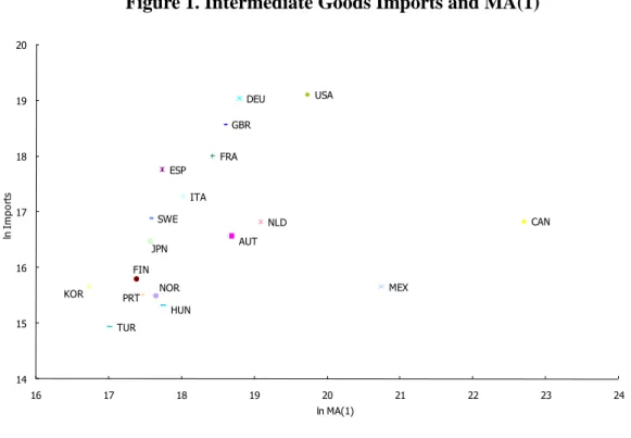
Figure 1. Intermediate Goods Imports and MA(1)
AUT CAN DEU ESP FIN FRA GBR HUN ITA JPN KOR MEX NLD NOR PRT SWE TUR USA 14 15 16 17 18 19 20 16 17 18 19 20 21 22 23 24 ln I m po rts ln MA(1) 6
We also tried the estimation method proposed by Helpman, Melitz, and Rubinstein (2008), which corrects for zeros in the trade matrix (export selection) and for the unobservable fraction of exporting firms (extensive margin). We use the product market regulation indices provided by the OECD Stat as excluded variables. Since our model does not have a large number of censored observations (just 3%), the coefficients for correcting for those two elements are not well identified and are insignificantly estimated, as is consistent with Belenkiy (2008). However, the standard explanatory variables have significant coefficients, which are almost the same as those in the case of the simple OLS and Tobit: Dist (-0.938), Language (0.965) and NAFTA (4.430).
25
4.2. Gravity for Intermediate Goods
MAr is calculated using (7) and the OLS result from Section 4.1. Mean values of
country r‟s imports of intermediate goods during 1997-1999 are plotted against the
means of calculated MAr in Figure 1. Three-letter codes (see Appendix) are used to
indicate each country. Excluding two outliers (Canada and Mexico), there is a clear positive relationship between a given country‟s access to the total demand for finished goods and its imports of intermediate goods. Eliminating the two outliers, an approximated straight line drawn on the sample has a slope of 1.03, and this is close to the theoretical prediction of unity. The extraordinarily high market access of outliers is reconsidered in Section 4.3.
Substituting predicted values of MAr into equation (6), the gravity equation for
intermediate goods may be estimated. Unlike trade in downstream goods, there are few observations in the sample (only two) with zero-value trade in upstream products. Thus, after adding the value of one to all intermediate goods trade before taking logarithms, only OLS results are reported in column (I) in Table 2.
Estimates of coefficients for the importer‟s access to the total demand for finished goods and the exporter production of intermediate goods are significantly positive. Thus, imports of intermediate goods appear sensitive not only to the magnitude of importer demand for finished goods but also to its neighbors‟ demand. The coefficient for exporter production of intermediate goods is near unity; this is also consistent with theoretical prediction. Estimated coefficients in the trade cost function are significant with the expected sign. As usual in studies of gravity, short distance and common language between trading partners increase trade in intermediate goods.
26
Table 2. Gravity Estimation for Intermediate Goods Trade
(I) (II) ln Zsr ln (Zsr/Zs) Dist -1.135*** -1.155*** [-24.37] [-24.57] Language 0.871*** 0.826*** [5.15] [4.85] NAFTA 2.364*** 2.269*** [6.07] [5.78] Output (Zs) 0.927*** [23.90] Wages (wr) 0.644*** 0.641*** [6.41] [6.39] Wages (vs) 0.383*** 0.293*** [3.23] [3.10] Supplier Access (ηr) 0.237*** 0.238*** [11.78] [11.95] MA(1) 0.098*** 0.103*** [2.89] [3.03]
Year YES YES
Obs. 1,026 1,026
R-sq 0.6688 0.5314
Notes: MA(1) was calculated by making intra-national trade costs a function only of intra-national
distance, defined as 0.66*(surface areai/π)
1/2
. ***, ** and * indicate, respectively, 1%, 5% and 10% levels of statistical significance. Bootstrapped standard errors are in parentheses (200 replications).
NAFTA also contributes to expansion of trade among member countries. The coefficients for both importer‟s and exporter‟s wages are significantly positive. On one hand, the theoretically inconsistent result in exporter‟s wages may be due to the fact that wages also capture worker quality. In other words, since intermediate goods production seems to require workers to be more highly educated than those in finished goods production, the coefficient for exporter‟s wages might be estimated to be positive. On the other hand, the result in importer wages is due to our elimination of price index for intermediate goods by introducing the estimates of supplier access. That is, the possible negative relationship between intermediate goods trade and their price
27
index shows up in the result of importer wages. Finally, the coefficient for the supplier access index is significantly positive. Theoretically, this result implies that the elasticity of substitution may be small in intermediate goods or large in finished goods, or that the linkage between finished and intermediate goods is strong.
In order to address the above-mentioned simultaneity problem, ln Zs may be
moved to the left side of the equation. The result is reported in column (II) of Table 2 and is virtually unchanged relative to (I). These results indicate that the simultaneity problem between trade and production is not so serious. Specifically, the estimated coefficient for MA is significantly positive.
4.3. Modifying DMA
Figure 1 shows that estimates of MAs in Canada and Mexico are extraordinarily large. It seems unnatural that these would be larger than MA in the US. Thus, calculation of MA is modified with particular attention to those three countries.
The first modification involves balancing DMA and FMA. The mean values of MA(1) and DMA(1) during the sample period are reported in column (I) in Table 3. It is natural that DMA in the US would be larger than that in Canada and Mexico. However, the average DMA is evaluated much lower than FMA. Such low evaluation could be one source of the extraordinarily large MAs in Canada and Mexico. The low evaluation may also be partly attributable to taking the commonality of language into account only in inter-national trade costs despite the fact that the same language is spoken within a nation. Based on this, intra-national trade costs and the method of calculating DMA may be modified as follows:
rr
r rr
r rrr Dist Language Dist
28
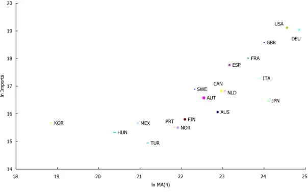
Figure 2. Intermediate Goods Imports and MA(4)
AUS AUT ESP FIN FRA GBR HUN ITA JPN KOR MEX NOR SWE TUR CAN DEU NLD PRT USA 14 15 16 17 18 19 20 18 19 20 21 22 23 24 25 ln MA(4) ln Im port s
The modified DMA(2) is reported in column (II) of Table 3. Compared with DMA(1), the modified version of DMA increases. However, MA(1) is much larger in Canada and Mexico than in the US because DMA(1) on average is still much lower than FMA.
Further investigation reveals that there are two sources for such low values of DMA(2). One is the evaluation of intra-national distance. Under the definition that Distrr = 0.66*(surface areai/π)1/2, intra-national distance in the US (around 1,000 km)
becomes larger than inter-national distance between the US and Canada (around 500 km). Obviously, it is unnatural that Canadian producers have better access to US demand for finished goods than US producers. Thus, as in Redding and Venables (2004), intra-national distance may be set to 100 km in any country. DMA may then be calculated as follows:
29
Table 3. Mean Market Access during Sample Period
ln FMA ln MA(1) ln DMA(1) ln MA(2) ln DMA(2) ln MA(3) ln DMA(3) ln MA(4) ln DMA(4) ln MA(4) ln DMA(4) ln FMA
AUS 15.7 16.0 14.6 16.5 15.9 18.6 18.5 22.9 22.9 23.1 23.1 12.2 AUT 18.5 18.7 16.7 19.0 18.0 19.1 18.1 22.5 22.5 20.2 20.1 18.5 CAN 22.7 22.7 13.0 22.7 14.4 22.7 17.1 23.0 21.5 21.5 21.3 19.7 DEU 18.0 18.8 18.2 19.8 19.6 20.5 20.5 24.9 24.9 24.7 24.7 18.7 ESP 17.4 17.7 16.3 18.3 17.7 19.0 18.8 23.2 23.2 22.3 22.3 16.2 FIN 17.2 17.4 15.5 17.7 16.8 18.2 17.7 22.1 22.1 19.5 19.5 16.6 FRA 18.2 18.4 16.7 18.9 18.1 19.5 19.2 23.6 23.6 22.4 22.3 18.9 GBR 18.1 18.6 17.5 19.3 18.9 19.8 19.6 24.0 24.0 24.3 24.3 18.1 HUN 17.7 17.7 14.4 17.8 15.8 17.9 15.9 20.4 20.3 19.2 19.1 17.0 ITA 17.3 18.0 17.3 18.9 18.7 19.6 19.5 23.9 23.9 24.1 24.1 16.4 JPN 15.5 17.6 17.4 18.9 18.8 19.7 19.7 24.1 24.1 23.0 23.0 11.9 KOR 16.7 16.7 12.6 16.8 14.0 16.9 14.2 18.9 18.6 18.7 18.6 14.2 MEX 20.7 20.7 11.5 20.7 12.9 20.7 14.7 20.9 19.1 20.6 20.6 15.3 NLD 18.8 19.1 17.5 19.6 18.9 19.4 18.7 23.1 23.0 22.8 22.7 20.3 NOR 17.5 17.6 15.3 17.9 16.7 18.2 17.5 21.9 21.9 20.0 19.9 17.0 PRT 17.2 17.5 15.9 18.0 17.3 18.0 17.4 21.8 21.8 20.5 20.4 16.0 SWE 17.4 17.6 15.5 17.9 16.9 18.4 17.9 22.3 22.3 22.5 22.5 16.3 TUR 17.0 17.0 14.1 17.2 15.5 17.6 16.8 21.2 21.2 19.6 19.6 15.5 USA 19.7 19.7 16.1 19.8 17.5 20.7 20.2 24.6 24.5 23.8 23.8 17.2 (V) Extended Sample
(I) (II) (III) (IV)
OECD Sample
Notes: DMA(1) is calculated by setting intra-national trade costs as a function of only intra-national distance (defined as 0.66*(surface areai/π)
1/2
). DMA(2) is calculated using a function of not only the intra-national distance (as in (I)) but also Languageii, (further set to unity). DMA(3) is calculated using a
function of intra-national distance (set to 100 km in any country), and Languageii, (set to unity). In DMA(4), intra-national trade costs are assumed to be a
30
rr
r
r rrr Dist Language
DMA (3) ˆ1exp ˆ2 exp ˆ 100ˆ1exp 1ˆ2exp ˆ
Column (III) in Table 3 reports results of DMA(3) and shows a large increase in the US. As a result, US MA(3) reaches a similar level to that of Mexico but is still much lower than that of Canada.
Another reason for DMA being lower than FMA is that Canada still gets better access to US markets than the US producers because of benefits from NAFTA. Thus, the last modification incorporates NAFTA effects into intra-national trade costs. FTAs are one means of moving member countries to an integrated or borderless economy. In this sense, the benefits of intra-national trade should be at least as large as the benefits of trade among FTA members. Therefore, the last modification of the calculation of DMA(4) is as follows.
r r rr rr rrr Dist Language NAFTA
DMA ˆ exp 1 exp 1 exp 100 ˆ exp exp exp ) 4 ( 3 2 1 3 2 1 ˆ ˆ ˆ ˆ ˆ ˆ
NAFTArr=1 for any country r. The results are provided in column (IV). The
relationship between MAr(4) and intermediate goods imports may also be seen in
Figure 2. As a result, US MA(4) exceeds both Mexican MA(4) and Canadian MA(4) due to the remarkable rise of DMA(4).
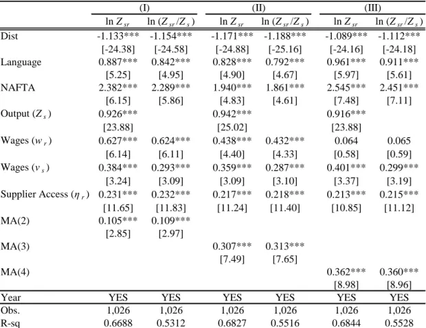
Using these three measures of DMA, equation (6) may again be estimated. Regression results are reported in Table 4 and are almost unchanged from those in Table 2. It is interesting that the coefficient of MA rises gradually. Since the theoretically predicted magnitude of the MA coefficient is unity, its rise implies that the modified measure of MA is more appropriate. However, the coefficient for the best measure of MA (MA(4)) is still far from unity (around 0.36). Thus, a more sophisticated measure of MA is needed, especially in the treatment of the intra-national
31
trade cost function.
Table 4. Gravity Estimation for Intermediate Goods Modifying DMA
ln Zsr ln (Zsr/Zs) ln Zsr ln (Zsr/Zs) ln Zsr ln (Zsr/Zs) Dist -1.133*** -1.154*** -1.171*** -1.188*** -1.089*** -1.112*** [-24.38] [-24.58] [-24.88] [-25.16] [-24.16] [-24.18] Language 0.887*** 0.842*** 0.828*** 0.792*** 0.961*** 0.911*** [5.25] [4.95] [4.90] [4.67] [5.97] [5.61] NAFTA 2.382*** 2.289*** 1.940*** 1.861*** 2.545*** 2.451*** [6.15] [5.86] [4.83] [4.61] [7.48] [7.11] Output (Zs) 0.926*** 0.942*** 0.916*** [23.88] [25.02] [23.88] Wages (wr) 0.627*** 0.624*** 0.438*** 0.432*** 0.064 0.065 [6.14] [6.11] [4.40] [4.33] [0.58] [0.59] Wages (vs) 0.384*** 0.293*** 0.359*** 0.287*** 0.401*** 0.299*** [3.24] [3.09] [3.09] [3.10] [3.37] [3.19] Supplier Access (ηr) 0.231*** 0.232*** 0.217*** 0.218*** 0.213*** 0.215*** [11.65] [11.83] [11.24] [11.40] [10.85] [11.12] MA(2) 0.105*** 0.109*** [2.85] [2.97] MA(3) 0.307*** 0.313*** [7.49] [7.65] MA(4) 0.362*** 0.360*** [8.98] [8.96]
Year YES YES YES YES YES YES
Obs. 1,026 1,026 1,026 1,026 1,026 1,026
R-sq 0.6688 0.5312 0.6827 0.5516 0.6844 0.5528
(I) (II) (III)
Notes: MA(2) is calculated as a function not only of intra-national distance (defined as
0.66*(surface areai/π)
1/2
), but also Languageii (further set to unity). MA(3) is calculated using a
function of intra-national distance (set to 100 km in any country) and Languageii, (set to unity). In
MA(4), intra-national trade costs are assumed to be a function of intra-national distance (set to 100 km in any country), Languageii, and NAFTAii, (both set to unity). ***, ** and * indicate,
respectively, 1%, 5% and 10% levels of statistical significance. Bootstrapped standard errors are in parentheses (200 replications).
4.4. Simulation
Using the model developed earlier, we simulate the impact of finished goods market expansion in a country on intermediate goods trade through input-output relationships
32
between those two types of goods. The simulation scenario includes the rise of US
final demand (λUS in 1999) by 10%. This increases finished goods exports of each
country to the US immediately. To produce such finished goods in a given country, the country must import intermediate goods from the world. As a result, world trade in intermediate goods experiences an explosive increase. For simulation, the impact of the finished goods market expansion in the US on intermediate goods trade is
quantified using the case of ln Zsr in column (III) in Table 4. Specifically, differences in
predicted values in the original case and the above-mentioned scenario are calculated.
Results are reported in Table 5. Firstly, the rise of λUS directly increases market
access in each country. Obviously, such an increase becomes more significant in countries that have lower trade costs with the US. Except for the US, Canada experiences the most remarkable increase in MA, with Mexico following. Secondly, in spite of the expansion of US demand only for finished goods, the increase in intermediate goods imports can be observed in all countries. This is a consequence of
the model with input-output relationships.7 The larger increase in Canadian imports
over US imports is due to the great number of imports of intermediate goods from the US. Thirdly, exports increase in all countries. As mentioned just above, most of the US exports of intermediate goods go to Canada, and vice versa.
7
This is also based on a property of the CES production function and thus is a different force from the „magnification effect‟ found in Yi (2003).
33
Table 5. Simulation: Impact of a 10% Rise in the US Market (US$1,000)
MA(4) Imports Exports AUS 599 6 1,042 AUT 379 43 817 CAN 1,884,473 3,867,567 1,610,208 DEU 432 12 15,723 ESP 1,817 93 7,337 FIN 390 21 196 FRA 448 27 9,127 GBR 1,888 150 14,299 HUN 367 43 173 ITA 374 9 3,371 JPN 228 3 25,868 KOR 895 1,299 3,926 MEX 261,777 177,283 38,869 NLD 446 85 842 NOR 441 22 299 PRT 485 22 338 SWE 411 37 991 TUR 315 10 144 USA 11,990,024 1,700,210 4,013,371 Total 14,146,189 5,746,942 5,746,941
Notes: This table shows the results of the simulation of a 10% rise in the US market (λUS) and uses
the result obtained in the case of ln Zsr in column (III) in Table 4. Changes in MA(4), total imports
of intermediate goods, and exports are reported.
4.5. Further Robustness Checks
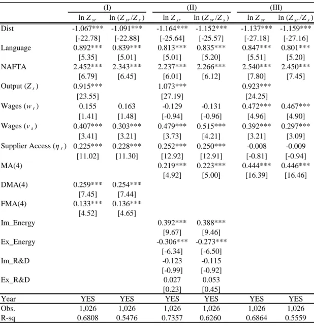
Further estimations may be made using DMA and FMA as separate terms. Theoretically, this regression is not well specified, but it may still be valuable for examining the validity and significance of importer demand (DMA) and its neighbors‟ demand (FMA) separately. Results are reported in column (I) in Table 6. The coefficient for importer‟s wages turns out to be insignificant. Estimated coefficients for both DMA and FMA are significantly positive, and this indicates that not only the importing country‟s demand for finished goods but also its neighbors‟ demand for finished goods are significantly important for trade in intermediate goods. The
34
magnitude of the estimated coefficient is a little larger in DMA than in FMA.
More control variables may also be added. Heretofore, only wages were introduced as a proxy for primary production factor prices. In order to control the effects of other primary factors, logs of importer and exporter energy production (Ex_Energy, Im_Energy; kilo ton of oil equivalents) and a share of R&D expenditures in GDP (Ex_R&D, Im_R&D) are added. This data is from the World Development Indicators (World Bank). Results are reported in column (II) of Table 6. While the coefficient for importer‟s wages is again insignificant, that of MA(4) is still significantly positive though with reduced magnitude. Results for the newly-added variables were disappointing. One reason for such results would be the high correlation among those variables.
Finally, sample countries are extended in the estimation of the gravity equation for finished goods trade. Although the sample in the gravity equation for intermediate goods was restricted to OECD countries due to availability of data, it is important to incorporate demand emanating from non-OECD countries in the calculation of the market access measure. For example, the present measure in Japan does not incorporate access to Chinese demand despite the fact that it is one of the most important markets for Japanese finished goods producers. Thus, not only OECD countries but also non-OECD countries are included in the sample for first stage
estimation (sample countries increase from 19 to 49).8
8
The following countries were added: Argentina, Bulgaria, Brazil, Switzerland, Chile, China, Colombia, Costa Rica, Cyprus, Estonia, Greece, Guatemala, Hong Kong, Croatia, India, Ireland, Iran, Israel, Kenya, Lebanon, Lithuania, Malta, New Zealand, Poland, Romania, Russian Federation, Singapore, Slovenia, Uruguay and Vietnam.
35
Table 6. Gravity Estimation for Intermediate Goods Trade: Robustness Checks
ln Zsr ln (Zsr/Zs) ln Zsr ln (Zsr/Zs) ln Zsr ln (Zsr/Zs) Dist -1.067*** -1.091*** -1.164*** -1.152*** -1.137*** -1.159*** [-22.78] [-22.88] [-25.64] [-25.57] [-27.18] [-27.16] Language 0.892*** 0.839*** 0.813*** 0.835*** 0.847*** 0.801*** [5.35] [5.01] [5.01] [5.20] [5.51] [5.20] NAFTA 2.452*** 2.343*** 2.237*** 2.266*** 2.540*** 2.450*** [6.79] [6.45] [6.01] [6.12] [7.80] [7.45] Output (Zs) 0.915*** 1.073*** 0.923*** [23.55] [27.19] [24.25] Wages (wr) 0.155 0.163 -0.129 -0.131 0.472*** 0.467*** [1.41] [1.48] [-0.94] [-0.96] [4.96] [4.90] Wages (vs) 0.407*** 0.303*** 0.479*** 0.515*** 0.392*** 0.297*** [3.41] [3.21] [3.73] [4.21] [3.21] [3.09] Supplier Access (ηr) 0.225*** 0.228*** 0.252*** 0.250*** -0.008 -0.009 [11.02] [11.30] [12.92] [12.91] [-0.81] [-0.94] MA(4) 0.219*** 0.223*** 0.444*** 0.446*** [4.92] [5.00] [16.39] [16.46] DMA(4) 0.259*** 0.254*** [7.45] [7.44] FMA(4) 0.133*** 0.136*** [4.52] [4.65] Im_Energy 0.392*** 0.388*** [9.67] [9.46] Ex_Energy -0.306*** -0.273*** [-6.34] [-6.50] Im_R&D -0.123 -0.115 [-0.99] [-0.92] Ex_R&D 0.027 0.053 [0.23] [0.45]
Year YES YES YES YES YES YES
Obs. 1,026 1,026 1,026 1,026 1,026 1,026
R-sq 0.6808 0.5476 0.7357 0.6260 0.6864 0.5559
(II) (III)
(I)
Notes: The sample used in the first stage estimation in column (III) includes not only OECD but
also non-OECD countries as well. ***, ** and * indicate, respectively, 1%, 5% and 10% levels of statistical significance. Bootstrapped standard errors are in parentheses (200 replications).
36
Figure 3. Intermediate Goods Imports and MA(4): Extended Sample
A U S A U T CAN D E U E S P F I N F R A G B R H U N I T A J P N KOR M E X NLD N O R S W E TUR U S A P R T 14 15 16 17 18 19 20 18 19 20 21 22 23 24 25 l n M A ( 4 ) ln Im port s
Results with this extended sample are as follow.9 Column (V) in Table 3 shows
the calculated MA, DMA, and FMA. Figure 3 depicts the relationship of MA with imports of intermediate goods. This table and figure show that US MA again exceeds both Mexican and Canadian MA. However, new estimates in the first-step gravity equation with the extended sample yield a lower MA in most countries than before. Gravity results in intermediate goods trade are reported in column (III) of Table 6. While the coefficient for supplier access turns out to be insignificant, estimates of MA are again significantly positive, and magnitudes are larger when compared with those in Table 4. The latter result may indicate the importance of incorporating the demand of as many countries as possible in the calculation of the market access measure.
9
As in Table 1, OLS regression in the first stage yielded significant coefficients for Dist (-2.44), Language (1.74) and NAFTA (1.44).
37
5. Concluding Remarks
This paper examined the role of importer‟s access to the finished goods market in intermediate goods trade by estimating the gravity-like equation derived from the NEG model. Specifically, we regress a gravity equation for finished goods trade in the first step. Then, introducing importer‟s access to demand for finished goods, which is calculated by using the estimates in the first step, we regress our gravity equation for trade in intermediate goods. As a result, we found that imports of intermediate goods are sensitive not only to the magnitude of the importer‟s demand for finished goods but also to that of its neighboring countries‟ demand. Based on the regression result, we also simulate the impact of the rise in US consumers‟ demand for finished goods on intermediate goods trade in each country. The simulation shows that, in spite of the expansion of US demand not for intermediate goods but rather for finished goods, an increase in intermediate goods imports can be observed in all countries, particularly in countries that have lower trade costs with the US.
38
Appendix: Sample Countries
3-letter Country Name AUS Australia AUT Austria CAN Canada FIN Finland FRA France DEU Germany HUN Hungary ITA Italy JPN Japan
KOR Korea, Republic of MEX Mexico NLD Netherlands NOR Norway PRT Portugal ESP Spain SWE Sweden TUR Turkey GBR United Kingdom
39
References
Amiti, M., 2005, Location of Vertically Linked Industries: Agglomeration versus Comparative Advantage, European Economic Review, 49(4): 809-832.
Ando, M. and Kimura, F., 2005, The Formation of International Production and Distribution Networks in East Asia, In: Ito, T., and Rose, A. (Eds.). International Trade (NBER-East Asia Seminar on Economics, Volume 14), The University of Chicago Press.
Athukorala, P.-C. and Yamashita, N., 2006, Production Fragmentation and Trade Integration: East Asia in a Global Context, The North American Journal of Economics and Finance, 17(3): 233-256.
Baier, S.L. and Bergstrand, J.H., 2001, The Growth of World Trade: Tariffs, Transport Costs, and Income Similarity, Journal of International Economics, 53(1): 1-27. Baier, S.L. and Bergstrand, J.H., 2007, Do Free Trade Agreements Actually Increase
Members‟ International Trade?, Journal of International Economics, 71(1): 72-95.
Belenkiy, M., 2008, Robustness of the Extensive Margin in the Helpman, Melitz and Rubinstein (HMR) Model, MPRA Paper 17913, University Library of Munich, Germany.
Bosker, M. and Garretsen, H., 2008, Economic Geography and Economic Development in Sub-Saharan Africa, CESifo Working Paper Series CESifo Working Paper No. 2490, CESifo Group Munich.
Brakman, S., Garretsen, H., Schramm, M., 2006, Putting New Economic Geography to the Test: Free-ness of Trade and Agglomeration in the EU Regions, Regional
40
Science and Urban Economics, 36: 613-635.
Combes, P.-P., Mayer, T., and Thisse, J.-F., 2008, Economic Geography, Princeton University Press.
Egger, H. and Egger, P., 2005, The Determinants of EU Processing Trade, World Economy, 28(2): 147-168.
Feenstra, R., 2002, Border Effects and the Gravity Equation: Consistent Methods for Estimation, Scottish Journal of Political Economy, 49(5): 491-506.
Hayakawa, K. and Kimura, F., 2009, The Effect of Exchange Rate Volatility on International Trade in East Asia, Journal of the Japanese and International Economies, 23(4): 395-406.
Head, K. and Mayer, T., 2000, Non-Europe: The Magnitude and Causes of Market Fragmentation in the EU, Review of World Economics/Weltwirtschaftliches Archiv, 136(2): 284-314.
Head, K. and Mayer, T., 2004, Market Potential and the Location of Japanese Investment in the European Union, Review of Economics and Statistics, 86(4): 959-972.
Head, K. and Mayer, T., 2006, Regional Wage and Employment Responses to Market Potential in the EU, Regional Science and Urban Economics, 36(5): 573-594. Helpman, E., Melitz, M., and Rubinstein, Y., 2008, Estimating Trade Flows: Trading
Partners and Trading Volumes, Quarterly Journal of Economics, 123(2): 441-487.
Hering, L. and Poncet, S., 2009, The Impact of Economic Geography on Wages: Disentangling the Channels of Influence, China Economic Review, 20(1): 1-14. Kheder, S.B. and Zugravu, N., 2008, The Pollution Haven Hypothesis: a Geographic
41
Economy Model in a Comparative Study, FEEM Working Paper No. 73.2008. Kimura, F., Takahashi, Y., and Hayakawa, K., 2007, Fragmentation and Parts and
Components Trade: Comparison between East Asia and Europe, The North American Journal of Economics and Finance, 18(1): 23-40.
Knaap, T., 2006, Trade, Location, and Wages in the United States, Regional Science and Urban Economics, 36(5): 595-612.
Krugman, P., 1991, Increasing Returns and Economic Geography, Journal of Political Economy, 99(3): 483-499.
Mayer, T., Mejean, I., and Nefussi, B., 2007, The Location of Domestic and Foreign Production Affiliates by French Multinational Firms, Working Papers 2007-07, CEPII research center.
Pagan, A., 1984, Econometric Issues in the Analysis of Regressions with Generated Regressors, International Economic Review, 25(1): 221-247.
Redding, S. and Schott, P., 2003, Distance, Skill Deepening and Development: Will Peripheral Countries ever Get Rich?, Journal of Development Economics, 72(2): 515-541.
Redding, S. and Venables, A.J., 2004, Economic Geography and International Inequality, Journal of International Economics, 62(1): 53-82.
Rose, A.K., 2004, Do We Really Know That the WTO Increases Trade?, American Economic Review, 94(1): 98-114.
Yi, K-M., 2003, Can Vertical Specialization Explain the Growth of World Trade?, Journal of Political Economy, 111(1): 52-102.
![Table 1. Gravity Estimation for Finished Goods Trade OLS Tobit Dist -1.087*** -1.095*** [0.139] [0.135] Language 1.388*** 1.408*** [0.302] [0.329] NAFTA 4.385*** 4.385*** [0.678] [0.733]](https://thumb-ap.123doks.com/thumbv2/123deta/9896280.1373133/16.892.311.575.201.448/table-gravity-estimation-finished-goods-trade-tobit-language.webp)