Model Adaptation based on HMM decomposition for Reverberant Speech Recognition

全文

(1)M ODEL ADAPTATION BAS ED ON H乱1M DECOMPOSITION FOR REVERBERAN T SPEECH RECOGNITION. TetJuya TAKIGUCHl1. SatoJhi. N AK AMU RA 1. Kiyohiro SH1 K A N 01. Qiaπ9 HU02. 1Graduate Sch∞1 of Information Science，Nara Institute of Science and Technology 8916-5 Takayama Ikoma，Nara， 630・01 JAPAN. 2 ATR Interpreting Telecommunications Research Labs.. 2-2，Hikaridai，Seika-cho，Soraku-gun，Kyoto 619・02，Japan E-mail: tetuy-t@is.aist-nara.ac.jp. ABSTRACT. The performance of a speech recognizer is degraded dras. tically in reverberant environments. We proposed a novel. algorithm which c祖 model an observation signal by com. position of HMMs of clean speech， noise and an acoustic transfer function[1]. However，how to estimate HMM pa rameters of the acoustic transfer function is a remaining se. rious problem. In our previous paper[1]， we measured real. impulse response吉of training positions in an experiment. room. It is inconvenient and unrealistic to measure impulse responses for every possible new experiment room. This pa. per presents a new method to estimate HMM parameters. of the acoustic transfer function from some adaptation data by using an HMM decomposition algorithm which is an in. verse process of the HMM composition. 1 ts effectiveness is. confìrmed by a series of speaker dependent and independent. word recognition experiments on simulated distant-talking speech data.. to recognition of the signal which is contaminated by not. only additive noise but also reverberation. If signal sources are independent each other and additive，the HMM compo. sition algorithm c回 be adopted. Noise and speech are as. sumed to be independent and additive in the time domain. While an acoustic transfer function and speechむe convo・. lutional in the time domain， they are assumed to be inde. pendent and additive in the cepstral domain. We showed effectiveness of the proposed method[1] through the recog. nition experiments for noisy reverberant speech. However，. how to estimate HMM parameters of an acoustic transfer function is a remaining serious problem. In our previous. paper[ 1]， we measured real impulse responses of the 紅白n. ing positions in the testing room. The me祖vectors of姐 acoustic transfer function HMM are derived仕om measured. impulse responses. However， it is inconvenient and unre. alistic to measure impulse responses for the testing room every time.. This paper presents a new method to estimate HMM. parameters of the acoustic tr阻sfer function based on the 1.. INTRODUCTION. In hands-free speech recognition， one of the key issues to. HMM decomposition. The proposed algorithm is obtained as the natural result of a reverse process of the HMM com. position. It can be applied to estimate the parameters of the. practical use is the development of a technology which en. acoustic transfer function HMM efficiently by using some. technology will play an especially important role in the. measured impulse responses.. 血姐y works have been performed in HMMs，and their train. 2.. ables ac四rate recognition of noisy reverber叩t speech. This. recognition of dist回t-talking speech. In the past few years，. ing algorithms to improve the speaker independent speech. recognition accuracy. To achieve a high recognition accu. racy，a user usually must equip with a close-talking micro. phone.. If a speaker inputs hisfher speech from the dis. adaptation speech data from the user's location instead of. This section presents 回 overview of the HMM composition. algorithm.. ment noise. Many methods have b田n proposed to cope with the problems caused by additive noise and convolu tional distortion. Among them， speech enhancement and. model compensation approaches are two examples. For the speech enhancement approach，spectral subtraction for ad. ditive noise 祖d cepstral mean normalization for convolu. The observation signal in a noisy reverberant. room is modeled by. tance or through a telephone channel，the recognition ac curacy will seriously degrade due to the infiuences of re verberation or telephone channel distortion and environ. HMM COMPOSITION. 。(t). =. S(t) . H(t) + N(t).. We assume that clean sp田ch and noise are independent，. and cle担speech and an acoustic transfer function are con volutional. Since the signal processing for the speech recog. nition are normally based on the short time spectral anal ysis，we regard O(t)，S(t)，N(t) as short time linear spectra whose analysis window starts at time t from now on.. H(t). is short time linear spectrum of the acoustic transfer func・. tional distortion had been proposed (e.g.，[2，3，4]). For the model compensation approach，conventional multi-template. tion.. been developed.. stochastic information sources are additive. To apply the. technique，model adaptation (e.g.，[9，10]) as well as model (de-)composition methods (e・E・， [1，5，6，7，8，11， 12]) had In our previous paper. [1]， we apply the HMM composは10n. 0-8186-7919-0/97 $10.00 ll:) 1997 IEEE. 1 t is also denoted to be a function of t because we. assume that the speaker may move around in a room.. The HMM composition algorithm is applicable if two. HMM composition，the equation can be rewritten as follows. 827. 53.

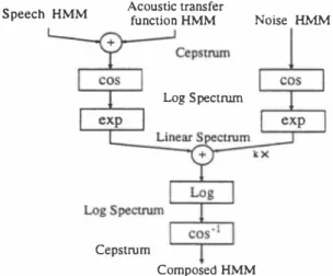
(2) 1.. in the cepstral doma.in: 1 Oce，，(t) = .F- (log(exp(.F(Sc叩(t) +Hc叩(t))) +N( t))). 1 Here， .F， .F- are Fourier(cosine) transform and inverse Fourier(cosine) transform，respectively. Accordingly a com. Re-estimate parameters of a composed HMM Moc.p using adaptation data in the noisy reverberant room by ML (maximum likelihood) or MAP (maximum a pOjte九ori)[13] estimation in the cepstral doma.in.. 2. Estimate parameters of a noise HMM MNc• p from the signal during noise periods.. posed HMM of the observation signal in the cepstral doma.in. is represented by. 3.. 1 Moc.P = .F- (log(exp(.F(Msc•p EÐ MHc•p)) EÐ kMNlin)).. Convert Moc.P MNc•p to the linear spectral doma.in: '. =exp(.F(Moccp))'. MO'.n. Here， M represents an associated HMM model; cep and lin represents the cepstral domain and the linear spectral. MN，川= exp(.F(MNccp ))'. doma.in respectively; k is a coefficient to adjust SNR; and EÐ denotes the model composition procedure. The model. 4. Decompose MSHlin from Molin:. composition is carried out as follows: The number of states. =MOlin e kMN';n'. MSHlin. and transition probabilities of composed HMMs become a product of number of states and transition probabilities of. Here， e denotes deconvolution of distributions. If the distributions can be represented by Gaussian distribu. each component model. The state observation probability. density functions (PDFs) of composed HMMs are obta.ined by the convolution of the two associated distributions. If the distributionsむeGa凶sians，say， N(μ1，σn，N(μ ，(7i)， their 2 convolution is still a Gaussian of N(μ1+μ ， (7; +σi). The 2 HMM composition procedure is schematically summarized. tion， N(μ， (72) C 回 be deconvolved into two distribu tions which are N(μ1，σÎ) 回d N(μーμ1，(72 -σÎ). 5. Convert MSHlin to the cepstral doma.in: 1 MSHc叩= .F- (log(泊SH';n))'. in Figure 1.. Acoustic transfer function HMM. Speech HMM. 6. Decompose MHc•p from MSHccp:. Noise H長仏4. MHccp = MSHccp e Msc. P ・ Here， MHccp is averaged over all distributions，りates and phone models based on theぉsumption that MHc<p is the same over the adaptation speech. It is also as. Log Spectrurn. sumed that MHccp is a one-state HMM having a single Gaussian with a diagonal covariance matrix. A tied. mixture HMM is used to model each speech unit in our experiments. The means. jj. and variances ü2 of庇Hcep. will be calculated as follows:. β. Cepstrum Composed HMM. {三μ=}. =乞乞7jI)AI)，. HMM DECOMPOSITION. 1=1・=1. If the structures of a noise HMM and 回 acoustic transfer. L. 5. ( M. 62=ZZ7jI){乞iλi弘(記1m-d，m). function HMM are given， the parameters of the individual. HMM can be estimated by a decomposition process. How ever， MN will usually be obtained separately， since noise HMM parameters c姐 be estimated accurately from the sig. +入日午(. nal during noise periods. The estimation equation of the acoustic transfer function HMM is rewritten as follows in. … _ jj.�1))2] } ，. ，(1) ， .... M ，， (1) ーで mμ_，m_ m -ん.m-μI，m anaμ，-Z m=l入.. (ん.m，記.m)臼d (μ..m，(7;.m) are (mean， vari組問). where μ ，. the cepstral doma.in:. 1 MHc叩= .F- (log( exp(.F(Moc•p)) e k exp(.F(MNc•p)) )). .l. of mth distributions of MSHccp and Msccp respec・ tively. Here (μ'，Tr\ ， σ;.m) = (μ.'，m，σ:，，m)，s#s'，since. 。Msc.P・. 必SHccp組d Ms ccpare tied mixture HMMs. 入i!L is the mixture coefficient of mth distribution of 8th state. Then the HMM decomposition procedure to estimate M H is described as follows:. of lth speech unit which keeps fixed during adaptation.. 828. 54. さ註さ刊dIり恰). =ささÎ�'). Figure 1. Block Diagram of HMM C o mp o siti o n. 3.. =.

(3) L is the number of speech units existed in adaptation data and S is the number of state of each sp四ch unit.. "Y�'. 90. ). is the weighting coefficient which is a ratio of the total number of frames belonging to state S of speech. � 80. data.. '"』. unit 1 over the total number of frames of the adaptation. 4.. g. 9 70 c 。" 0 ιJ U -. EXPERIMENT5 AND RE5ULT5. Recognition experiments are conducted to evaluate effec. tiveness of the proposed method. 1n this study， as a fìrst step， we focus on room reverberation distortion only and. 60. examine the decomposition of MH目p. =. o. 1. 2 3 4 5 10 Number of adaptation words. 50. MSHc•p e Msc.p' Figure 3.. 3. tal room. The sound signal is captured by using a single. 札一 P 一白 A 一. method reported in [14J. The length of reverberation time. 3. is approximately 180 msec for the experiment room.. 3. む. .3200. 品ヨ凶一回. 11 p1 [1 b1. 匂雪. Stocbastic-Match. 3. omni-directional microphone. We measured 9 transfer func tions corresponding to 9 sound source positions by using the. 智IIMicro向。ne. 5D and 51 word recognition rates[%] by. HMM adaptation. ‘ ‘ 、、、、 ?j 日山 ω 初 'A 叩日 n v nu 'a・ U E E 』』副島 S E R-咽。一時国己主〈. The decomposition of MSHlin from MOlin C担be dealt with separately. Figure 2 shows a top view of the experimen. p2回 b2 11. o. 6. 8. 10. 12. Figure 4. Convergence ofthe adaptation algorithms for 51 seed model. Figure 2. A top view of the experimental room. •. how the proposed methods work in both the 50 回d. the 51 recognition of reverberant speech.. performance of the composed model adaptations which. include ML and MAP reestimation.. Two speech corpora are used for evaluation. One is the A. •. set of the ATR Japanese speech database. The other is the. performance differences between the proposed meth. ods and other two popular techniques， na.mely ML. A5J continuous speech database. The former contains word utterances 回d the latter contains sentence utterances， both. database. The speaker dependent (50) model is trained by using 2620 words of two male and one female speakers from the ATR database， respectively. 500 words for testing are. 4. Number of iterations. •. spoken by 組nouncers. The speaker independent (51) model is trained by using utterances from 64 speakers in the A5J. 2. stochastic matching(5M)[9J and cepstral me回subtrac tion (CM5 ) [3J. Figure 3 shows 500・word recognition results averaged over. two male and one female speakers.. 'Adap-ML' refers to. the results by using the proposed method where composed model adaptation is carried out via ML reestimation， while. different from those used in SD training. The adaptation. 'Adap-MAP' is that of its MAP counterpart.. excluded from testing set. Each set of the adaptation word consists of 50 words. The test and adaptation data are simulated by linear convolution of clean speech signal and. are 79.8% and 66.5%， respectively. The 'Adap-ML' and 'Adap-MAP' improves the SD recognition rate to 87.6% and. words are also selected from those used in training， and. measured impulse responses from the positions p1，... ，p4. 54 context independent phone models are used. Each. phoneme HMM is a left-tcトright 3・state tied-mixture HMM. There are in total 2 56 Gaussian mixture components with. diagonal covariance matrices. Each feature vector consists. of 16 mel-frequency cepstral coe伍cients (MFCCs). A single Gaussi回 POF is used to model 回 acoustic transfer func・. tion for each position. A series of comparative experiments. are conducted to examine:. The aver. aged 5D and 51 recognition rates with clean speech HMMs. 86.2%， and the 51 recognition rate to 68.9% and 70.1% by. using 5 ada.pta.tion words in the average of the three speak ers， respectively. The result also shows that the 'Adap MAP' method is able to rapidly adapt the model param eters of the acoustic transfer function HMM by MAP es・. tima.tion， whereas in the 50 recognition， 'Adap-ML' out. performs 'Adap-MAP' when more adaptation data become. available. This is because with the 50 seed model， we c叩. get a more accura.te alignment for 50 ada.ptation data. Fur. thermore， '5tochastic-Match' refers to the result by using. 829. 55.

(4) the ML stochastic matching method ( SM)[9)， the recogni Table 1. Comparison of several methods. Clean. 11. Adap-ML. Adap-MAP. Ergodic-CHMM CMS. Stochastic-Match. SD. 79.8%(77.8%). II. 87.6%(84.3%). 86. 2%(83.1%). (86.2%). ( 75.2%). 86.8% (83.5%). ( ) indicates result for one speaker.. SI. 66.5% 68.9%. 70.1%. tion rates of the proposed 'Adap-ML ' method is slightly. higher than that of the SM method for the SD model， whereas it is worse than the SM method for the SI model. As future works， we need a model compensation pro. cedure that acts over much longer intervals th回 the tra ditional assumptions of the short-time stationarity of the speech signal.. 73.0%. the SM method[9]. The experimental results show that the. recognition performance of the 'Adap-ML' is slightly better. th回(or no big difference from) that of the SM method in. the SD seed model case， whereas the SM method achieves. a better perform祖ce th回the proposed methods in the SI. When more than one sources of distor. tion exist， e.g.， both additive and convolutional distortions，. some new theoretical frameworks are required to directly. take into account the nonlinear interaction between differ. ent types of distortions. When the distortion sources are non-stationary， e.g.， a moving speaker and a non-stationary. ambient noise， some adaptive compensation techniques are. needed. To enhance the efficacy and the effectiveness of the. compensation， those techniques むe mostly wanted to be able to better characterize the distribution of the poss・，ble. seed model case. One possible explanation for the latter ob. distortion types，臼d use this distribution to ch∞se the Ìl.p. that each state of the re-trained HMM corresponds to the associated state of the SI HMM is too fragile in the SI case.. lines of thoughts.. proposed 'Adap-ML' method and the SM method in the SI. [IJ. servation is that the assumption of the proposed methods. ln Figure 4， we compare the convergence property of the. propriate compensation model. We are working along these. REFERENCES tics distorted speech recognition by HMM compo.ition，"， Proc. seed model c笛e. The average log-likelih∞d per frame of one adaptation word versus iteration number of EM algo・. ICASSP・96，. rithm is plotted. The results show that one or two iterations. [2J. Table 1 summarizes the performance comparison of sev. [3J. seem enough for both algorithms.. eral methods for the SD and the SI recognition experi ments. In this table， 'Clean' is the result by using the mod. els trained on clean speech. 'Ergodic・CHMM' is the result. tion HMM constructed from 5 training positions， h1，. . . ，hs・. 'CMS' is the result of the cepstral me阻 subtraction [3ト In this case， the SD seed model is trained by using CMS. recognition rate from 79.8% to 87.6% by using 5 adaptation. words without血y measurement of impulse responses. The. [4J. [5] [6]. [8]. the proposed methods improve the SD recògnition rate from. 1992， pp.233・236.. M. J. F. Gale.， S. J. Young，“PMC for speech recognition in a.ddi. by. è:omposition. of. hidden. Markov. models，"，. Proc.. 1993， pp.l031・1034.. A. Sa.nka.r and C.・H. Lee， “Robust speech recognition based on atochastic ma.tching，" Proc. ICASSP-9S，. 1995， pp.121・124.. V. Abrash， A. Sanka.r， H. Fra.nco and M. Cohen， “Acoustic a.da.ptation using tra.nsformations of HMM pa.ra.meters，". ICASSP-96，. [11]. 1993.. F. Martin， K. Shika.no a.nd Y. Minami， “Recognition of noi.y. EUROSPEECH-93，. Proc.. 1996， pp.729・732.. Y. Minami日d S. Furui，吐血山田um likelihood procedure for a. universaJ a.da.ptation method based on HMM composition，". Proc. ICASSP-9S，. [12]. 1995， pp.129・132.. Y.Mina.mi and S. Furui， “Ada.ptation method based on HMM composition. and. EM. algorithm，". Proc.. ICASSP96，. 1996，. pp. 327・330.. [13]. C.-H. Lee， C.-H. Lin and B.・H. Juang， “A study on speaker adaptation. of. the. parameters. of. continuous. density. hidden. Ma.rkov models，" IEEE Tran.. on Signal Proce..ing， Vol. No.. [14]. 39，. 4， pp.806-814， 1991.. Y. Suzuki， F. Asano， H.-Y. Kim， a.nd T. Sone， “An optimum computer-generated pulae sign&l叫ita.ble for the measuremeot of. 79.8% to 87.6%， and the SI recognition rate from 66.5% to. very long impulse re.pon.es，". 70.1 % for reverberant speech by using 5 adaptation words. No.. in the average of the three speakers. In comparison with. 830. 56. M. J. F.Gales and S. J. Young， “An improved a.pproa.ch to the. speech. sured impulse responses but by the adaptation data from. the user's location. The experimental results indicate that. 1990， pp.845・848.. tive a.nd convolutiona.l noi.e，" CUED-F-INFENG-TRI54，. eters of 回 acoustic transfer function based on the HMM. rameters of the acoustic transfer function HMM not by mea. 1990.. A. P. Va.rga. and R. K. Moore，官idden Ma.rkov model decomposi・. ICASSP-92，. [7]. ation time as 180 msec in this study. On the other hand，. decomposition. These methods enable to estimate the pa. A. Acero， Acou.tical and Environmental Robu.tne.. in Auto. hidd四Markov model decomposition of speech and no凶e，" Proc.. ant speech recognition， especially with such a long reverber. We have presented a new method to estimate HMM param. 55， pp.1304・1312， 1974.. tion of speech and noi.e，"， Proc. ICASSP-90，. [10J. DISCUSSION AND CONCLUSION. Acou.t. Soc. Amer.， Vol.. matic Speech Recognition， Ph.D Dissertation， ECE Depa.rtment，. [9]. 5.. 1979.. B. Atal， “E宵ectiveness of linear p日dictioo characteri.tics of the. CMU， Sept.. that the simple CMS technique does not work in reverber. improve the performance somehow.. S. F. Boll，“Supp日泊四n of acoustic noise in speech using .pectral. " J.. performance for one speaker is only slightly (1.9%) worse than that of an ergodic transfer function HMM where real impulse responses are used. The result also clearly shows. both the proposed methods and the SM method are able to. pp.69・72.. .peech wave for automatic speaker identification and verification，. processed clean speech data. The results in Table 1 show. that our proposed 'Adap-ML ' method improves the SD. 1996，. subtraction，" IEEE Tran.. on ASSP， Vol. ASSP-27， No.2，. by using the previously proposed [1) composed model of a clean speech HMM and 姐 ergodic acoustic 仕組sfer func. S. Nakamura， T. Takiguchi， K. Shikano，“Noise and room acous. 2， pp.1l19-1123， 1995. J.. Acou.t. Soc. Amer.， Vol.. 97，.

(5)