HUSCAP Journals

Instructions for use

T itle Higher Multiplicity in the One-D imensional A llen-C ahn A ction F unctional

A uthor(s ) R eznikoff,Maria G; T onegawa,Y oshihiro

C itation Hokkaido University Preprint S eries in Mathematics, 821: 1-55

Is s ue D ate 2006-12-15

D O I 10.14943/83971

D oc UR L http://hdl.handle.net/2115/69629

T ype bulletin (article)

Higher Multiplicity in the One-Dimensional

Allen-Cahn Action Functional

Maria G. Reznikoff,

and Yoshihiro Tonegawa

December 15, 2006

Abstract

We prove the Γ-convergence of the Allen-Cahn action functional in the sharp-interface limit. In previous work, good lower bounds were developed under the assumption of single-multiplicity, but the bounds deteriorated in the case of higher-multiplicity interfaces. We develop improved bounds by working directly with the limiting energy measures.

Contents

1 Introduction 2

1.1 Rare events in stochastic differential equations . . . 7

1.2 Analysis of the sharp-interface limit . . . 9

1.2.1 Summary of previous results for the action functional . 11 1.2.2 Progress and method . . . 13

1.3 Remarks and notation . . . 15

1.4 Proof of Lemma 1.2 . . . 20

1.5 Organization . . . 21

2 The upper and lower bounds 21 2.1 Proof of Theorem 1.1 . . . 21

2.2 Proof of Proposition 1.1 . . . 24

2.2.1 Proofs of Lemmas . . . 26

3 Propagation estimate 29

3.1 Proof of Proposition 3.1 . . . 31

3.2 From single multiplicity to higher multiplicity . . . 36

3.2.1 Proof of Lemma 3.3 . . . 37

3.3 Proof of Proposition 3.2 . . . 42

3.4 Proof of Auxiliary Lemmas . . . 47

3.4.1 Proof of Lemma 3.1 . . . 47

3.4.2 Proof of Lemma 3.2 . . . 50

3.4.3 Proof of Lemma 3.4 . . . 51

3.4.4 Proof of Lemma 3.5 . . . 52

Keywords: Allen-Cahn equation, stochastic partial differential equations, large deviation theory, action minimization, sharp-interface limits, Γ-convergence. AMS Subject Classification Numbers: 49J45, (35R60, 60F10).

1

Introduction

In this paper we complete the analysis of the sharp-interface limit (ε→0) of the functional

Sε(u) =

1 4

Z T

0

Z 1

0

εu˙2+ε−1(εuxx−ε−1V′(u))2dx dt, (1.1)

where for simplicity we choose the standard potential

V(u) = (1−u

2₎2

4 . (1.2)

(The analysis can be carried out for any nondegenerate double-well potential

V, changing only the value of the constantc0 defined below.) The work in [18]

stopped short of a complete analysis because of the issue of multiplicity in the limiting energy. We now resolve that issue.

The functional Sε will be defined on the space:

A=nu∈C∞([0,1]×[0, T])|u(·,0)≡ −1, u(·, T)≡+1,

ux(0, t) =ux(1, t) = 0

o .

In order to introduce the limit functional and space, we need to introduce some measures. Let

M := nmeasuresµon [0,1]_×[0, T]¯¯ ¯µ=

Z T

0

dµtdt

and∃ {Tk}Mk=1 ={0≤T1 < . . . < TM ≤T}

such that∀t /∈ {Tk}Mk=1, µt=c0

N(k)

X

j=1

δgj(t)

where 0≤g1(t)≤. . .≤gN(k)(t)≤1, sup

k

N(k)<∞,

andgj ∈C((Tk, Tk+1)), g˙j ∈L2((Tk, Tk+1))∀j, k

o .

Notice that the pointsgj are allowed to be equal; we say thatgjhas multiplicity

J if J is the maximal number such that there exists a set _{gi+1, . . . gi+J} ∋gj

with

gi+1 =gi+2 =. . .=gi+J.

Let

µTk+ = lim

t↓Tk

µt, µTk− = lim

t↑Tk

µt,

where we set by definition

µt = 0 fort <0 or t > T, (1.3)

so that in particular µT−

1 = µT +

M = 0.For µ∈ M, define

SM(µ) = 1 2

M

X

k=1

¯ ¯ ¯µ

T+

k −µTk−

¯ ¯ ¯

T V +

c0

4

M−1

X

k=1

Z

(Tk,Tk+1)

N(k)

X

j=1

( ˙gj)2dt. (1.4)

Here_{| · |}T V denotes the total variation norm and the constant c0 denotes

c0 =

Z +1

−1

p

2V(u)du (1.2)= 2

√

2 3 .

In some sense, (1.4) represents the limit of (1.1), but although the functional

Sε is defined on functions, the limiting object SM is defined on measures.

For the usual Γ-convergence framework, we would like instead to measure the limiting cost in terms of the function u to which a sequence {uε} converges.

We make that connection below.

x=1 x=1 T2

T3

T1= 0

T4=T

Figure 1: The figure on the left depicts a function u(x, t) that is equal to +1 in the shaded regions and ₋1 outside. A measure µu that is supported only

at the discontinuities of u incurs a cost at T2 and T3 in the first term of SM.

A measure µ that has a multiplicity two interface for t _∈(T2, T3) as depicted

in the figure on the right, however, incurs no such cost.

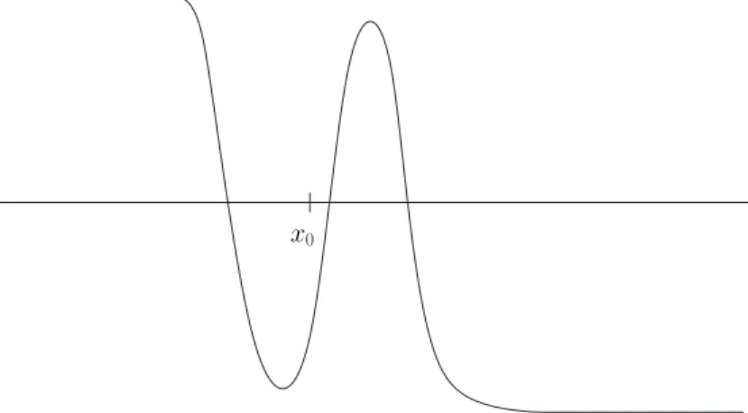
x0

Figure 2: A sequence _{uε} in which three interfaces accumulate at the same

pointx0 in the limitε→0 leads to a multiplicity three delta mass atx0. (See

Definition 1 (Admissible functions). We call the function u0 : [0,1]×

[0, T]→R admissible if

(i) The function u0 = ±1 a.e. and the number of jump discontinuities of

u0(·, t) is uniformly bounded.

(ii) The boundary between a region of u0 = +1andu0 =−1is a continuous

function of time. (More precisely, the boundary of u0 = +1 is contained by

the graphs of finitely many continuous functions of time.) (iii) For any x0 ∈[0,1] and r >0, the function

m(_{x_∈Br(x0)|u(x, t) = +1})

is a continuous function of time. Here m(A) denotes Lebesgue measure and

Br(x0) denotes a ball of radius r around x0.

(iv) The function satisfies u0(·,0)≡ −1 and u0(·, T)≡+1.

From [18] it follows:

Lemma 1.1. For any sequence of functions uε ∈ A such that Sε(uε) is

uni-formly bounded, there exists a subsequence and a limit function u0 such that

u0 is an admissible function and

lim

ε→0_t∈sup_[0,T]||uε(·, t)−u0(·, t)||L

2_([0,1]) = 0.

Therefore it makes sense to consider the set of admissible functions. We associate to each admissible u the measures µu that are compatible in the

following sense.

Definition 2 (Compatible measures). Supposeu(_·, t) =_±1a.e. andu(_·, t)

has jump discontinuities 0 < y1 < y2 < . . . < yn(t) < 1. We say that the

measure µu ∈ M is compatible with u if

(a) For all t /∈ {Tk}Mk=1,

{yj}nj=1(t) ⊂ {gj}Nj=1(k).

(b) At points where µu has a delta mass with odd multiplicity, uhas a jump

discontinuity, and at points where µu has a delta mass with even multiplicity,

u has no jump discontinuity.

We define

A0 =

n

uis admissible and there exists a compatible measure µu ∈ M

Notice that for a given function u_{∈ A}0, there are many compatible measures

µu. We will show the Γ-convergence of Sε to the functional S0 : A0 → R

defined via:

S0(u) := inf

µu

SM(µu). (1.5)

In other words, the limit functional chooses the “best” admissible measure. See Figure 1 for an example in which the best measure isnot just the one with delta masses at the discontinuities of the limit function.

There are two ingredients for the Γ-convergence. The first is:

Proposition 1.1 (Upper bound). For everyu0 ∈ A0, there exists a sequence

uε ∈ A with uε →u0 in L∞(L2) such that

lim sup

ε→0 Sε(uε) ≤ S0(u0).

We prove Proposition 1.1 in Section 2. The first task is to show that the infimum in (1.5) is attained; the rest of the proof relies on reducing to the construction from [17].

The lower bound is subtle since it requires proving that no sequence can do better than the constructions used in Proposition 1.1. In [18], a lower bound is proved under the assumption of single-multiplicity. This assumption prohibits different interfaces of the finite ε problem from accumulating at the same position in the limitε _→0; cf. Figure 2 and the discussion in Subsection 1.2.2. In this paper we prove the lower bound with no extra assumptions:

Theorem 1.1 (Lower bound). Given any sequence uε ∈ A with

lim sup

ε→0

Sε(uε) < ∞ and uε →u0 inL∞(L2),

we have that u0 ∈ A0 and moreover,

lim inf

ε→0 Sε(uε) ≥ S0(u0). (1.6)

1.1

Rare events in stochastic differential equations

Ordinary differential equations. The Wentzell-Freidlin theory of large deviations [12] links the study of “rare events” with the variational problem of action minimization, as we now explain. Consider the finite-dimensional stochastic gradient flow

˙

X = _−∇V(X) +p2γB˙ t >0, (1.7)

X = x− t= 0,

whereX _∈Rn_{, ˙B represents white noise, andV is a double-well potential with}

minima x− and x+. Under the deterministic dynamics (γ = 0) x− is stable, but under noisy dynamics (γ >0) the solution is eventually driven out of the basin of attraction ofx− and intoBǫ(x+), a ball of radius ǫaroundx+. Let B

denote the set of functions that “switch” in time T,

B:=nx¯¯x(0) =x₋, x(T)∈B_ǫ(x₊) o

.

Wentzell-Freidlin theory estimates the exponential factor in the probability of switching as

lim

γ→0 γ log Prob

¡

X _{∈ B}¢

= ₋inf_{S(x)_|x_{∈ B}}, (1.8)

where S(_·) is the so-called large deviation action functional,

S(x) = 1 4

Z T

0 |

˙

x+_∇V(x)_|2dt. (1.9)

Notice that the minimization problem on the right-hand side of (1.8) is deter-ministic.

In addition to estimating the probability of switching, large deviation the-ory estimates the mechanism of switching. Suppose that x∗ _{is the unique} minimizer of S overB. Then for anyδ >0,

lim

γ→0

Prob³X _{∈ B}and dist(X, x∗_{)< δ}´

Prob³X ∈ B´ = 1.

Partial differential equations. Large deviation theory generalizes to the case of infinite-dimensional stochastic gradient flows, i.e., stochastically per-turbed partial differential equations. The simplest interesting example of a stochastic PDE that is well-posed and for which the large deviation action functional has been identified is the stochastic Allen-Cahn equation,

˙

U = Uxx−V′(U) +

p

2γη t >0, x_∈[0, L], (1.10)

U = u− t= 0, x∈[0, L],

whereη is a space-time white noise and u− is an energy minimizer; see below. Assume for simplicity that V is the standard double-well potential,

V(u) = (1−u

2₎2

4 .

The deterministic PDE (i.e., γ = 0) is the L2 _{gradient flow for the energy}

functional

E(u) =

Z L

0

1 2(ux)

2_{+V(u)dx, (1.11)}

which admits two global minimizers u− and u+ (as long as L ≥ 2π). For

Neumann or periodic boundary conditions u± ≡ ±1 ; for Dirichlet boundary conditions u± ≈ ±1 on most of [0, L] with modification near the boundary. For simplicity, we will focus in this section on homogeneous Dirichlet boundary conditions.

Faris and Jona-Lasinio [9] prove that

S(u) = 1 4

Z T

0

Z L

0

( ˙u−uxx+V′(u))2dx dt (1.12)

is the action functional for the Allen-Cahn equation onC₀−, the space of con-tinuous functions on [0, L]×[0, T] withu(0, t) =u(L, t) = 0 and u(·,0) = u−, with the topology inherited from the sup norm.

In analogy with the finite dimensional system (1.7), u− is stable under the deterministic dynamics, but for γ > 0 there is a positive probability of switching to Bǫ(u+), a ball of radius ǫ around the symmetric minimum. Let

B denote the set of functions in C₀− that transform in time T:

B:=nu¯

¯u(0, t) =u(L, t) = 0, u(·,0) =u₋, u(·, T)∈B_ǫ(u₊) o

. (1.13)

Notice thatB is a “regular set” in the sense of Wentzell and Freidlin [12], i.e.,

inf

In particular, it follows from [9] that

lim

γ→0γ log Prob

¡

U _{∈ B}¢

= ₋s. (1.15)

As in the finite dimensional case, we have in addition that action minimizers are the most-likely switching pathways. We do not expect the action minimizer to be unique, so let us define

B∗ :={u|u∈ B, S(u) = s}. (1.16)

(Here _B denotes the closure of _B.) From the work of Faris and Jona-Lasinio [9] it follows:

Lemma 1.2. The set _B∗ is nonempty and for any δ >0,

lim

γ→0

Prob³U _{∈ B} and dist(U,_B∗)< δ

´

Prob³U ∈ B´ = 1. (1.17)

We include a proof of Lemma 1.2 at the end of the introduction. Now we turn to the analysis of the action functional. For an interpretation of our results in terms of the stochastic equation see Remark 5 in Subsection 1.3.

1.2

Analysis of the sharp-interface limit

Because the action minimization problem is complicated, it is natural to ask whether there are limiting regimes in which the analysis simplifies. It is well-known that for the finite-dimensional problem in the limit T _{→ ∞}, the most-likely pathway is the one that follows the time-reversed gradient flow

˙

x = _∇V(x)

to flow from x− to the saddle point with lowest energy, and the forward gra-dient flow

˙

x = −∇V(x)

to flow from this saddle point to Bǫ(x+). Faris and Jona-Lasinio proved that

the same holds for the infinite dimensional problem [9]. This saddle-point problem that controls the action minimization problem in the long-time limit

T → ∞is important; indeed, if phase transformation is studied on the natural time-scale of the system, then this pathway is the most likely.

events are physically relevant: For instance they explain phenomena observed in magnetic switching experiments [19]. They are also analytically interesting: We will see that a competition between the time- and length-scales of the system leads to a family of action minimizing pathways with increasing spatial structure.

Introduction of the sharp-interface limit. We consider the action func-tional in the limit L _{→ ∞}, T _{→ ∞}, L/√T = constant. (For a general discussion of the different parameter regimes of the action problem, see [17].) Letting ε := 1/L, x _→ εx, t _→ ε2_{t, and T → ε}2_{T, (1.12) can be reexpressed}

as:

Sε(u) =

1 4

Z T

0

Z 1

0

³

ε1/2u˙ +ε−1/2(εuxx−ε−1V′(u))

´2

dx dt, (1.18)

where we have grouped terms in order to isolate

fε(u) := εuxx−ε−1V′(u),

the first variation of the rescaled energy

Eε(u) =

Z 1

0

ε

2(ux)

2₊V(u)

ε dx. (1.19)

Recall the boundary conditions

ux(0, t) = ux(1, t) = 0 (1.20)

and the initial and final conditions

u(x,0) =u−, u(x, T) = u+. (1.21)

(See Remark 2 in Subsection 1.3 for alternate formulations.) Notice that (1.21) implies

Eε(u(·,0)) = Eε(u(·, T)) = 0. (1.22)

Squaring the integrand of (1.18), using (1.20) to integrate by parts, and ap-plying (1.22), we arrive at the functional Sε defined in (1.1).

In addition, observe that for any sequence uε with action bounded by ¯C

and for any time t_≤T, we have

¯

C ≥ Sε(u) ≥

1 2

¯ ¯ ¯ ¯

Z t

0

Z 1

0

˙

u fε(u)dx dt

¯ ¯ ¯ ¯

(1.20),(1.22)

= 1

Hence the energy is uniformly bounded in time, and (1.19) implies that uε

must converge to±1 almost everywhere in space withsharp interfacesdividing regions of u = +1 from regions of u =₋1. The uniform energy bound (1.23) is critical for the analysis.

Related sharp-interface limits. The sharp-interface limit of the action functional Sε fits naturally into a “family” of sharp-interface problems that

are well-known in the calculus of variations and PDE communities. The con-vergence of the energy functional (1.19) to the perimeter functional was ana-lyzed in [21] (see also [20] and [25]). Subsequently, the sharp-interface limit of the gradient flow dynamics was investigated; see [3, 14, 2] for the case d = 1 and [24, 6, 7, 16] for the case d > 1. Another related problem in d > 1 is a conjecture of DeGiorgi on which there has been recent progress [23, 22] and which says, roughly speaking,

ε−1 Z

Ω

(ε∆u₋ε−1V′(u))2dx ⇀ c0

Z

Γ

κ2dσ,

where Γ is the interface and κ is the mean curvature. While closely related to these sharp-interface problems, the action functional is unique as a time-dependent variational problem.

1.2.1 Summary of previous results for the action functional

The numerical study of the sharp-interface limit of the Allen-Cahn action func-tional for d = 1,2 in [8] suggested two competing action costs: A nucleation cost to form interfaces, and a propagation cost to move them. (See also [11] ford= 1 and [17] for d≥1.) The numerically observed minimizers formed an optimal number N of interfaces at t = 0 and moved the interfaces across the system with constant velocity. It was observed that the optimal number of interfaces increases as the experiment timeT decreases, which was understood to reflect the fact that moving a single wall across the system in a short time incurs a high propagation cost.

To what degree can these observations be made rigorous? This question was raised in [18] (for d = 1). It was observed that insight into the action functional could be gained by exploiting earlier results on the time-independent problem

ε∆u₋ε−1_V′_{(u) = f}

ε,

where fε is a sequence of functions satisfying a given bound (cf. [15, 27, 26]).

Consider the energy measures defined by

dµε :=

µ ε

2(ux)

2₊ V(u)

ε ¶

dx dt, (1.24)

and the action measuresνε defined by

dνε :=

1 4

¡

εu˙2+ε−1f_ε2¢

dx dt. (1.25)

The first result is a continuity theorem for the limiting energy measures:

Theorem 1.2 (Continuity, Theorem 1.1 in [18]). Consider any sequence of smooth functions on [0,1] × [0, T] that have uniformly bounded action, bounded initial and final energy, and Neumann boundary conditions. Choose any subsequence such that the corresponding measures µε and νε converge as

measures to µ and ν in the limit ε→0. Let E be the set of times at which

η:=

Z

[0,1]

dν (1.26)

has a point mass. Then

(1) For all t in [0, T]_\E, µt

ε converges as a measure to a limit, µt.

(2) For all t in [0, T]\E, µt _{is continuous as a function of t with values in}

(W1,∞₎∗_.

(3) µ(Ψ) =RT

0 µ

t_{(Ψ)dt for all Ψ∈C([0, T]×[0,1]).}

The second result identifies the structure of the limit measures. It can be expressed:

Theorem 1.3 (Structure, Theorem 1.2 in [18]). For any subsequence as in Theorem 1.2, there exists a finite set of “singular times”

Tsing :={Tk}Mk=1 ={0≤T1 < T2, . . . < TM ≤T}

such that for all t_∈[0, T]_{\ T}sing,

µtε → ε→0 µ

t _{= c}

0

N(k)

X

j=1

δgj(t), (1.27)

where

0_≤g1(t)≤g2(t)≤. . .≤gN(k)(t)≤1. (1.28)

Here δgj is the delta-function at gj and N(k)<∞. Moreover,

Time-integrated equipartition of energy follows as a corollary:

Corollary 1 (Equipartition, Corollary 1 in [18]). Consider any subse-quence as in Theorem 1.3 and any interval[s, t]⊂[0, T] that does not contain any singular time of µ. Then

lim

ε→0

Z t

s

Z 1

0

ε

2(uε,x)

2_{dx dt}′ _{= lim}

ε→0

1 2

Z t

s

Z 1

0

µ ε

2(uε,x)

2₊ V(uε)

ε ¶

dx dt′.

As far as the action functional Sε, [18] identifies the limit of the minimum

value of the action, but stops short of a true Γ-convergence argument for the functional itself; see below.

1.2.2 Progress and method

In the case of higher multiplicity, the method of [18] produces too weak a lower bound. For an interface g of multiplicity J one expects the propagation cost to be J times that of a single-interface construction. Instead the lower bound from [18] is of the form

c0

J Z T

0

( ˙g)2dt.

While valid as a bound, it fails to capture the extra cost of moving a J -multiplicity wall.

The difficulty is that in order to get a sharp lower bound for the action functional one needs information about not just the limitfunction u0, but also

the limit measure µ. (The single-multiplicity assumption hides this difficulty since then u0 uniquely identifies the measure µ.) A loss of information in

the case of higher-multiplicity interfaces is familiar: In the case of the energy functional (1.19), the limiting energy is proportional to the multiplicity, but the perimeter functional (the Γ-limit) throws away this extra cost. To get a good bound for the action, however, we need to track the limiting energy measures, not just the perimeter.

The main ingredient for Theorem 1.1 is:

Proposition 1.2. Let_{uε}be any sequence of smooth functions with Neumann

boundary conditions and uniformly bounded action. Assume without loss that

µε and νε converge. Suppose that [0, T] contains no singular time.

Then the interfaces _{gj}Nj=1 are such that g˙j ∈L2([0, T])∀j = 1. . . N and

moreover,

c0

Z T

0

N

X

j=1

( ˙gj)2dt ≤ lim ε→0

Z T

0

Z 1

0

To illustrate the idea, we roughly sketch the argument for an isolated inter-faceg that has multiplicityJ on [0, T], so that in particular for any subinterval [t1, t2] we have

µt=c0J δg(t) ∀t ∈[t1, t2]. (1.30)

Notice also that by Corollary 1, we have

lim

ε→0

Z t2

t1 Z 1

0

ε(uε,x)2dx dt = c0J∆t, where ∆t:=t2−t1. (1.31)

Suppose thatgmoves monotonically to the right and let ∆g :=g(t2)−g(t1).

Define the piecewise linear test function:

φ(x) =

  

 

0 x < g(t1)

x₋g(t1) g(t1)≤x≤g(t2)

∆g x > g(t2)

and observe that

|φ′| ≤1 a.e. and |φ|∞ ≤∆g. (1.32)

We compute formally:

c0J∆g (1.30)

=

Z 1

0

φ dµt2

− Z 1

0

φ dµt1

= lim

ε→0

µZ 1

0

φ dµt2

ε −

Z 1

0

φ dµt1

ε

¶

= lim

ε→0

Z t2

t1 d dt

Z 1

0

φ³ε

2(uε,x)

2_+ε−1_W(u

ε)

´ dx dt

= lim

ε→0

Z t2

t1 Z 1

0

φ¡

εuε,xu˙ε,x+ε−1W′(uε) ˙uε

¢ dx dt

= lim

ε→0

Z t2

t1 Z 1

0

(₋φ′εuε,xu˙ε+φfεu˙ε)dx dt

≤ lim

ε→0

µZ t2

t1 Z 1

0

(φ′)2ε(uε,x)2dx dt

Z t2

t1 Z 1

0

ε( ˙uε)2dx dt

¶1/2

+1

2|φ|∞εlim→0

Z t2

t1 Z 1

0

ε( ˙uε)2+ε−1fε2dx dt

(1.32) (1.31) (1.26)

≤ µ

c0J∆tlim

ε→0

Z t2

t1 Z 1

0

ε( ˙uε)2dx dt

¶1/2

+ 2 ∆g Z t2

t1

The idea is that if η([t1, t2]) is small, then (1.33) gives

(c0J−δ)

(∆g)2

∆t ≤ limε→0

Z t2

t1 Z 1

0

ε( ˙uε)2dx dt

for some small δ >0. Taking a Riemann sum and letting δ_→0 leads to

c0J

Z T

0

( ˙g)2dt _≤ lim

ε→0

Z T

0

Z 1

0

ε( ˙uε)2dx dt.

In the actual proof, we will replace ∆g by the oscillation of g on subintervals and use the fact:

Lemma 1.3. Let g be any continuous function on [0, T]. Let Σ denote the family of all finite partitions σ of [0, T],

σ=_{0 =t0 < t1 < . . . < tn=T},

and

|σ_|:= max

0≤k≤n−1|tk+1−tk|.

Suppose that

lim

δ→0



 sup

σ∈Σ,

|σ|<δ n−1

X

k=0

(osc[tk,tk+1] g)

2

tk+1−tk





=:M < ∞.

Then g˙ _∈L2_{([0, T]) and}

Z T

0

( ˙g)2dt = M.

1.3

Remarks and notation

It is helpful to introduce some language.

Definition 3 (Multiplicity). Given an interface g : [0, T]→[0,1], the set

{Multg =J}

refers to the set of times t _∈ [0, T] for which J is the maximal number such that there exists a set of interfaces _{gℓ}jℓ+=Jj+1∋g with

gj+1(t) = gj+2(t) = . . .= gj+J(t).

We say that on this set g “has multiplicity J.” When we are referring to a group of J interfaces, we will sometimes shorthand

Definition 4 (Isolated group of interfaces). Let 1 _≤ j1 ≤ j2 ≤ N. We

will call {gj}jj2=j1 an isolated group of interfaces on (t1, t2) if there does not

exist t_∈(t1, t2) such that gj1−1(t) = gj1(t) or gj2(t) =gj2+1(t).

Definition 5 (Consecutive group of interfaces). By a consecutive group of J interfaces we will mean a set gj+1, gj+2, . . . , gj+J.

Remark 1 (Elementary bounds). We will often refer to the fact that if a sequence uε has uniformly bounded action, i.e.,

lim sup

ε→0

Sε(uε) ≤ C,¯

then it follows from (1.25) and (1.26) that:

Z T

0

dη ≤ C¯ (1.34)

and from (1.23) that

sup

t∈[0,T]

Eε(u(·, t)) ≤ 2 ¯C.

Remark 2 (Different initial and final conditions). The initial condition

u(_·,0) _{≡ −}1 in the definition of _A is not necessary. It can be replaced by a condition of uniformly bounded initial energy, or Sε(u) can be replaced by

Eε(u) +Sε(u).

We work with u(·,0)≡ −1for simplicity and because of the switching problem that motivates our study of the action functional.

One can also remove the end condition u(_·, T)_≡+1 and work instead with the original functional

Sε(u) =

1 4

Z T

0

Z 1

0

³

ε1/2u˙ +ε−1/2(εuxx−ε−1V′(u))

´2

dx dt. (1.35)

This form is more natural from a probabilistic point of view, but since we are working mainly with the variational problem we use (1.1) (which has an at-tractive symmetry). So that we can apply our results to the stochastic problem, let us consider how the sharp-interface limits of (1.35) and (1.1) are related.

In the sharp-interface limit of (1.35), the total variation in SM _{is replaced}

by

sup

0≤φ≤1

³

µTk+(φ)−µT

−

k(φ)

´+

where (_·)+ _{denotes positive part. This relies mainly on the fact that for any}

singular time Tj we have

Z Tj+δ

Tj−δ

Z 1

0

(ε1/2u˙ ₋εi−1/2fε(u))2dx dt

≥

Z Tj+δ

Tj−δ

Z 1

0

(ε1/2u˙ −ε−1/2fε(u))2φ(x)dx dt

≥ 4

à Z Tj+δ

Tj−δ

Z 1

0 −

˙

u fε(u)φ(x)dx dt

!+ .

(See [18], proof of Theorem 1.4.) Heuristically, (1.36) reflects that instead of paying half the nucleation cost to form or annihilate delta masses, one pays the full cost to form them and nothing to annihilate them.

The second term in the sharp-interface limit of (1.35) is the same as for

(1.1). To see that the propagation cost is unchanged, notice that on any interval

(t1, t2) containing no singular time, we have by Theorem 1.3 that µt([0,1]) is

constant for all t_∈(t1, t2). It follows in particular that

Z t2

t1 Z 1

0

(ε1/2u˙ +ε−1/2fε(u))2dx dt =

Z t2

t1 Z 1

0

ε( ˙u)2+ε−1(fε(u))2dx dt.

One modification is that with the end condition removed, we need to add

(TM, T) to the intervals over which we integrate in the second term on the

right-hand side of (1.4). Whenu(_·, T)_≡+1 is enforced, eitherT is a singular time or the interfaces have all annihilated at TM < T, so that there is no

prop-agation cost on(TM, T). Whenu(·, T)≡+1 is not enforced, T is by definition

never a singular time, however interfaces may propagate on (TM, T).

Remark 3 (Different boundary conditions). Neumann boundary condi-tions are simplest, but the Γ-convergence of the action functional can also be proved for the case of homogeneous Dirichlet boundary conditions. In this case the limit of the initial energy is c0 instead of zero, and µ0 consists of two delta

masses with weight c0/2 at x= 0 and x= 1.

Remark 4 (Minimizers are what we expect). The Γ-convergence of Sε

implies in particular that minimizing configurations are what we expect. Con-sider the limit problem

inf

u∈A0

S0(u).

x=1 x=1 t=T

g1=g2=g3

g2 g3

g1

Figure 3: When T is sufficiently small, achieving the minimal action re-quires three delta masses (cf. Remark 4). While [18] showed that the single-multiplicity configuration depicted on the left attains the minimal action (in this regime), it could not rule out the higher-multiplicity configuration de-picted on the right. Theorem 1.1 resolves this issue. Minimizing configurations

must have single-multiplicity and constant velocities. The only minimizers are the one shown on the left and its reflection.

numberN of jump discontinuities, which form att= 0 and move with constant velocity across the system (cf. Figure 3). Moreover, one expects the associated optimal measure to have single-multiplicity. While [18] showed that such a configuration achieved the minimal action, it did not show that this was the ONLY way to achieve the minimal action. In particular, it could not rule out higher-multiplicity configurations (cf. Figure 3, right-hand figure). The lower bound in Theorem 1.1 and the structure of SM _{reveal that indeed, optimal}

measures are what we expect: There is an optimal number N of delta masses (depending on T), and to minimize the second term in SM _{they must have}

single-multiplicity and move with constant velocity across the system.

functional (1.35) is the action functional corresponding to

εU˙ = εUxx −ε−1V′(U) +

p

2γεη. (1.37)

We can also obtain (1.37) by rescaling space and time in the S-PDE (1.10). In order to connect our results with the large deviation estimates of [9], con-sider the S-PDE with homogeneous Dirichlet boundary conditions. Fix T and lets0 denote the minimum of the limit action (modified according to Remarks 2

and 3 above). The large deviation estimate (1.15) and the Γ-convergence of

(1.35) imply that for the solution of (1.37) we have

s0−o(1)ε→0 ≤ −lim

γ→0γ log Prob

¡

U ∈ B¢

≤ s0+o(1)ε→0.

As far as the most-likely switching pathways, Lemma 1.2 says that trajecto-ries stay within a δ–neighborhood of action minimizers (in the sup norm), but it doesn’t tell us what the action minimizers are. The Γ-convergence of (1.35)

gives us a way to approximate switching trajectories. Consider a sequence of action minimizers u∗

ε with u∗ε → u∗ as ε → 0. Consider the corresponding

functions u˜ε → u∗ constructed as in Proposition 1.1 with modification for the

boundary conditions. Finally, consider the stochastic trajectories U that are within a δ-neighborhood of u∗

ε in the sup norm on [0, T]×[0,1]. Noting that

sup

t∈[0,T]||

U −u∗_ε||L2_([0,1]) ≤δ,

we observe that U is well-approximated by the constructions u˜ε in the sense

that

sup

t∈[0,T]||

U₋u˜ε||L2_([0,1])

≤ sup

t∈[0,T]||

U ₋u∗

ε||L2_([0,1])+ sup

t∈[0,T]||

u∗

ε−u∗||L2_([0,1])+ sup

t∈[0,T]||

u∗_−u˜

ε||L2_([0,1])

≤ δ+o(1)ε→0.

1.4

Proof of Lemma 1.2

Proof. As in Subsection 1.1 above, let C₀− denote the space of continuous functions on [0, L]_×[0, T] that satisfy u(0, t) = u(L, t) = 0 and u(_·,0) = u−, equipped with the sup norm. By [9, Proposition 6.3], we have for any C <∞

that

{u|S(u)≤C} is compact inC₀−. (1.38)

Consider the set _{B ⊂} C₀− defined in (1.13) and a minimizing sequence _{un}

in _B such that limn→∞S(un) = s, the minimal action, cf. (1.14). Since B is

a closed subset of a compact space, we can extract a convergent subsequence. Letu∗ _{denote the limit. By [9, Proposition 6.2],}

S(_·) is lower semi-continuous on C₀−. (1.39) Hence S(u∗_{) =s and B}

∗ defined in (1.16) is not empty.

We now turn to the proof of (1.17). SinceB is an open set inC0−, it follows

from [9, Theorem 6.1] that for every ζ > 0 there exists γ0 > 0 such that for

γ ≤γ0 we have

Prob(U ∈ B) ≥ Prob(U ∈ B) ≥ exp

µ −1

γ(s+ζ) ¶

. (1.40)

Next, we claim that for any δ >0, we have

¯

s := inf

u∈B

dist(u,B∗)≥δ

S(u)> s. (1.41)

Indeed, suppose to the contrary that there exists a sequence _{un} inB with

lim

n→∞S(un) = s dist(un,B∗) ≥ δ.

We may assume without loss that S(un) ≤ C and hence by (1.38), we can

extract a convergent subsequence. Let ¯u denote the limit. It follows that

dist(¯u,_B∗) _≥ δ. (1.42)

On the other hand, by (1.39) we have in particular

s _≤ S(¯u) _≤ lim

Hence (1.41) is established. Moreover, since

{u|u∈ B,dist(u,B∗)≥δ}

is a closed set in C₀−, it follows from [9, Theorem 6.1] that for every ζ > 0, there exists a γ0 >0 such that for γ ≤γ0 we have

Prob³U ∈ Band dist(U,B∗)≥δ´ ≤ exp

µ −1

γ(¯s−ζ) ¶

. (1.43)

Letζ <(¯s−s)/2. Then the combination of (1.43) and (1.40) implies (1.17).

1.5

Organization

We begin in Section 2 by proving the lower bound (Theorem 1.1) given Propo-sition 1.2. Then in Subsection 2.2 we prove the upper bound (PropoPropo-sition 1.1). The heart of the paper is Section 3, where we prove Proposition 1.2. The proof is by induction. We prove the base case (Proposition 3.1) in Subsection 3.1. The induction step requires more work: We illustrate the main idea in Subsection 3.2 by showing how to go fromJ = 1 to J = 2 (Lemma 3.3). Then in Subsection 3.3 we prove the induction step (Proposition 3.2). Finally, the proofs of the auxiliary lemmas appear in Subsection 3.4

2

The upper and lower bounds

2.1

Proof of Theorem 1.1

Given Proposition 1.2, the proof of Theorem 1.1 is straightforward and follows the method from [18].

Proof. Choose a subsequence such that

lim inf

ε→0 Sε(uε)

is attained. Choose a subsequence such that µε and νε converge as measures.

We consider separately the intervals [Tk − δ, Tk +δ] ∩[0, T] “near singular

times” and the intervals [Tk+δ, Tk+1−δ] “away from singular times,” where

δ >0 satisfies

δ < 1

Consider any interval [Tk −δ, Tk +δ]. Choose any φ ∈ C1([0,1]) with

0≤φ(x)≤1. We estimate:

1 4

Z Tk+δ

Tk−δ

Z 1

0

ε( ˙uε)2+ε−1(fε(uε))2dx dt

≥ 1 2 ¯ ¯ ¯ ¯

Z Tk+δ

Tk−δ

Z 1

0

˙

uε(εuε,xx−ε−1V′(uε))φ dx dt

¯ ¯ ¯ ¯

≥ 1₂ ¯ ¯ ¯ ¯

Z Tk+δ

Tk−δ

Z 1

0

(εu˙ε,xuε,x−ε−1u˙εV′(uε))φ dx dt

¯ ¯ ¯ ¯ − 1 2 ¯ ¯ ¯ ¯

Z Tk+δ

Tk−δ

Z 1

0

εu˙εuε,xφ′(x)dx dt

¯ ¯ ¯ ¯

. (2.1)

We observe that on the one hand,

lim

ε→0

Z Tk+δ

Tk−δ

Z 1

0

(εu˙ε,xuε,x−ε−1u˙εV′(uε))φ dx dt

= lim

ε→0

Z Tk+δ

Tk−δ

d dtµ

t ε(φ)dt

= lim

ε→0

³ µTk+δ

ε (φ)−µTεk−δ(φ)

´

= µTk+δ_(φ)−_µTk−δ_(φ),

and on the other hand, letting ¯C denote the bound on the action, we have

¯ ¯ ¯ ¯

Z Tk+δ

Tk−δ

Z 1

0

εu˙εuε,xφ′(x)dx dt

¯ ¯ ¯ ¯

≤ ||φ||C1

µZ Tk+δ

Tk−δ

Z 1

0

εu˙2_εdx dt

¶1/2µZ Tk+δ

Tk−δ

Z 1

0

εu2_ε,xdx dt ¶1/2

≤ ||φ||C1 p

4 ¯Cp2 ¯C2δ

= ||φ||C1 O ¡√

δ¢ .

Together with (2.1), this yields

lim

ε→0

1 4

Z Tk+δ

Tk−δ

Z 1

0

ε( ˙uε)2+ε−1(fε(uε))2dx dt

≥ 1₂¯¯µTk+δ(φ)−µTk−δ(φ) ¯

¯− ||φ||_C1 O(

√

Notice that the “boundary intervals” are special: For T1 = 0, the interval is

[0, δ] and recalling µ0

ε = 0∀ε, (2.2) becomes

lim

ε→0

1 4 Z δ 0 Z 1 0

ε( ˙uε)2+ε−1(fε(uε))2dx dt

≥ 1

2

¯ ¯µδ(φ)

¯

¯− ||φ||_C1 O(

√

δ)

= 1

2

¯

¯µδ(φ)−µ−δ(φ) ¯

¯− ||φ||_C1 O(

√

δ).

Similarly, for TM =T we have

lim

ε→0

1 4

Z T

T−δ

Z 1

0

ε( ˙uε)2+ε−1(fε(uε))2dx dt

≥ 1₂¯¯µT−δ(φ) ¯

¯− ||φ||_C1 O(

√

δ)

= 1

2

¯

¯µT+δ(φ)−µT−δ(φ) ¯

¯− ||φ||_C1 O(

√

δ).

Away from singular times, we will use Proposition 1.2. Consider any in-terval [Tk +δ, Tk+1 −δ]. Then gj for j = 1, . . . , N(k) are well-defined and

moreover by (1.29),

lim

ε→0

1 4

Z

(Tk+δ,Tk+1−δ) Z 1

0

ε( ˙uε)2dx dt ≥

c0

4

Z

(Tk+δ,Tk+1−δ)

N(k)

X

j=1

( ˙gj)2dt. (2.3)

Combining (2.2) and (2.3) and summing overk, we deduce

lim inf

ε→0

1 4 Z T 0 Z 1 0

ε( ˙uε)2+ε−1(fε(uε))2dx dt

≥ 1 2 M X k=1 ¯

¯µTk+δ(φ)−µTk−δ(φ) ¯ ¯+

c0

4

M−1

X

k=1

Z

(Tk+δ,Tk+1−δ)

N(k)

X

j=1

( ˙gj)2dt

−M_||φ_||C1 O(

√

δ).

Sending δ _→0 on the right-hand side gives

lim inf

ε→0

1 4 Z T 0 Z 1 0

ε( ˙uε)2+ε−1(fε(uε))2dx dt

≥ 1 2 M X k=1 ¯ ¯ ¯µ T+

k(φ)−µT

−

k (φ)

¯ ¯ ¯+

c0

4

M−1

X

k=1

Z

(Tk,Tk+1)

N(k)

X

j=1

and taking the supremum over 0_≤φ _≤1 yields

lim inf

ε→0

1 4

Z T

0

Z 1

0

ε( ˙uε)2+ε−1(fε(uε))2dx dt

≥ 1₂

M

X

k=1

¯ ¯ ¯µ

T+

k −µTk−

¯ ¯ ¯

T V +

c0

4

M−1

X

k=1

Z

(Tk,Tk+1)

N(k)

X

j=1

( ˙gj)2dt,

i.e.,

lim inf

ε→0 Sε(uε) ≥ S

M_(µ).

Since for all t /_{∈ {}Tk}Mk=1 the support of µ includes the discontinuities of u0

and delta masses have odd multiplicity whereu0 has a jump discontinuity and

even multiplicity otherwise, it follows thatµis an admissible measure and we have in particular that

lim inf

ε→0 Sε(uε) ≥ S0(u0).

2.2

Proof of Proposition 1.1

Proof. We begin with two simplifying lemmas. First we argue that the minimal action is attained:

Lemma 2.1. For every u0 ∈ A0 there exists a compatible measure µ∗ such

that

SM(µ∗) = inf

µu0

SM(µu0).

The idea is to build a constructionuεwithuε→u0 inL∞(L2) such that the

associated energy measures µε converge to the minimizing measure µ∗. The

basic building block is the construction from [17], however a new complication is that µ∗ may exhibit higher-multiplicity interfaces. We can reduce to the simpler case using:

Lemma 2.2. Any compatible measure µ with higher-multiplicity interfaces may be approximated by compatible measuresµα with single-multiplicity

inter-faces in (0,1) in such a way that

lim

α→0S

M_(µ

Hence given any u0 ∈ A0 we may assume that the compatible measureµ∗ minimizes SM _{and that its interfaces have single-multiplicity and take values} in (0,1). Now we follow the construction from [17]. We briefly sketch the main ideas.

First we build the construction locally around a pair of interfaces and then show that the localized constructions can be merged. (The interfaces appear and annihilate in pairs because of condition (iii) in Definition 1.) Suppose that a pair of interfaces appear at location x0 at time T1. Without loss, suppose

that u =₋1 near x0 just before T1 and u = +1 near x0 just after T1. Define

the “nucleated state”

un(x) =

   

  

tanh

µ

x₋x0+ℓ

√

2ε ¶

x_≤x0

tanh

µ

−x+x0+ℓ

√

2ε ¶

x≥x0,

where ℓ is a free parameter. We connectu =₋1 to un(x) at time t =T1 +τ

in the following way. If ℓ is not too large, then there is an orbit connecting it via the dynamics ε1/2_{u˙ = ε}−1/2_(εu

xx −ε−1V′(u)) to u = −1 in infinite time.

On [T1, T1+τ] we first interpolate from u =−1 to a point arbitrarily nearby

(in L2_{) and on this orbit. Then we follow the time-reversed gradient flow to}

un. (For annihilation of interfaces, we use instead the forward gradient flow.)

As in [17], one can check that the time required for such a pathway is of order

τ _∼εexp(cℓ/ε) and that for any toleranceβ >0 there exists such a path with action bounded by

c0+β =

1 2

¯ ¯ ¯µ

T1+ −µT1− ¯ ¯ ¯

T V +β.

Hence by choosingℓ ≪ε, we can reachunin a time τ ≪1 with a good action

bound.

To move the interface, we use

uε(x, t) =

   

  

tanh

µ

x−g1(t) +ℓ

√

2ε ¶

x≤x0

tanh

µ

−x+g2(t) +ℓ

√

2ε

¶

x≥x0,

whereg1(T1+τ) = g2(T1+τ) =x0. Then the second term in the integrand of

(1.1) vanishes identically and for the first we can show the bound

Z

(T1+τ,T2) Z 1

0

εu˙2dx dt ≤ c0

Z

(T1+τ,T2)

Sending τ _→0 as ε_→0, we find

lim sup

ε→0

Sε(uε) ≤

1 2

¯ ¯ ¯µ

T+

1 −µT1− ¯ ¯ ¯

T V +

c0

4

Z

(T1,T2)

( ˙g1)2+ ( ˙g2)2dt.

Consecutive interfaces can be added. The constructionuε is defined piecewise

from the midpoint between one pair of interfaces to the midpoint between the next pair. It remains to show that the discontinuities in uε,x at every time

can be smoothed with only a small action cost. We refer the reader to [17] for details.

2.2.1 Proofs of Lemmas

Proof of Lemma 2.1. Choose a minimizing sequence of compatible measures

µn such that

SM_(µ

n)↓S0(u0) as n→ ∞.

It follows from the definition of SM _{that the µ}

n are uniformly bounded, and

hence we may choose a subsequence that converges in the sense of measures to some limit,µ∗. Thatµ∗ is compatible withu0 follows from the fact thatu0

is admissible.

We will now argue that

SM(µ∗) = inf

µu

SM(µu). (2.4)

Let T = {T1, . . . , TM} and Tn ={T1n, . . . , TMnn} denote the singular times of

µ∗andµn, respectively. By the convergence ofµntoµ∗, we have thatTn → T.

Hence forc >0 sufficiently small and anyk_{∈ {}1, . . . , M_}, takingnsufficiently large implies that there are no singular times of µn on (Tk+δ, Tk+1−δ). Let

{g1, . . . , gN(k)}and{gn1, . . . , gnNn_(k)}denote the locations of the delta masses of

µ∗ and µn, respectively. From the convergence of µn it follows that Nn(k) =

N(k) and for each j _{∈ {}1, . . . , N(k)_}, gn

j converges uniformly to gj. Moreover

by the uniform boundedness of eachgn

j inW1,2, we may conclude thatgjn⇀ gj

weakly in W1,2_{. By the weak lower semicontinuity of the L}2 _{norm, it follows}

that

Z

(Tk+δ,Tk+1−δ)

N(k)

X

j=1

( ˙gj)2dt ≤ lim inf n→∞

Z

(Tk+δ,Tk+1−δ)

N(k)

X

j=1

( ˙gn

j)2dt (2.5)

This is the first half of the proof of (2.4).

Now consider an interval (Tk−δ, Tk+δ) around one of the singular times

the “boundary intervals.”) On this interval the measureµnhas singular times

Tn

k,1, . . . , Tk,Jn for someJ ≥1. By the convergence of µn, we have

νn := J

X

j=1

µ(T

n k,j)

+

n −µ

(Tn k,j)−

n ⇀ µT

+

k

∗ −µT

−

k

∗ .

Hence by the weak lower semicontinuity of the total variation with respect to measure convergence, it follows that

|µT +

k

∗ −µ

T−

k

∗ |T V ≤ lim inf n→∞ ¯ ¯ ¯ ¯ ¯ J X j=1

µ(T

n k,j)

+

n −µ

(Tn k,j)−

n ¯ ¯ ¯ ¯ ¯ T V

≤ lim inf

n→∞ J X j=1 ¯ ¯ ¯µ

(Tn k,j)

+

n −µ

(Tn k,j)−

n

¯ ¯ ¯

T V . (2.6)

The combination of (2.6) and (2.5) (repeated for each Tk∈ T) establishes

SM_(µ

∗) ≤ lim inf

n→∞ S M_(µ

n).

Sinceµn is a minimizing sequence of SM over the set of compatible measures,

this completes the proof of (2.4).

Proof of Lemma 2.2. Consider (Tk+δ, Tk+1−δ) where Tk is an arbitrary

sin-gular time of µ. We will separate the interfaces in the following way. Let

{gj}Nj=1 denote the delta masses of µt on this interval. Add to the set g0 ≡0

and gN+1 ≡1. To separate the interfaces, we introduce:

forj = 1, . . . , N, g˜j :=gj + min

½

α2,gj+1−gj

4

¾ φ

µ

gj −gj−1

α ¶

−min

½

α2,gj−gj−1

4

¾ φ

µ

gj+1−gj

α ¶

,

where φ(x) is a smooth function that satisfies

φ(0) = 1, 0_≤φ_≤1, _|φ′_{| ≤}2, and φ(x) = 0 for x_≥1. (2.7)

It is not hard to check that ifgj(t)6=gj+1(t), then ˜gj(t)6= ˜gj+1(t), while on the

procedure a finite number of times all of the interfaces have single multiplicity. We denote the new interfaces by {gα

j}Nj=1.

We repeat the procedure on each interval (Tk+δ, Tk+1−δ). To complete the

construction, we linearly interpolate between the original and new positions of the delta masses. More precisely, on [Tk, Tk +δ], we linearly interpolate

between

lim

t↓Tk

gj(t) and gjα(Tk+δ),

and similarly, on [Tk−δ, Tk], we linearly interpolate between

lim

t↑Tk

gj(t) and gαj(Tk−δ).

This completes the construction of _{gα

j} on [0, T] and hence of µα. It

remains to show that the associated action is close to that of µ. It is easy to see that

M

X

k=1

¯ ¯ ¯µ

T+

k −µTk−

¯ ¯ ¯

T V = M

X

k=1

¯ ¯ ¯µ

T+

k

α −µT

−

k

α

¯ ¯ ¯

T V .

Hence, it suffices to show

Z Tk+1−δ

Tk+δ

( ˙g_jα)2dt =

Z Tk+1−δ

Tk+δ

( ˙gj)2dt+o(1)α→0. (2.8)

Moreover, since the iterative separation scheme is completed in a finite number of steps, it is enough to show (2.8) for a single step in the scheme. We compute the derivative explicitly:

d dt˜gj

= ˙gj+α( ˙gj −g˙j−1)φ′1{α2_≤(g

j+1−gj)/4}

+

µ

1

4( ˙gj+1−g˙j)φ+ 1

4α(gj+1−gj)( ˙gj −g˙j−1)φ

′

¶

1{0<(gj+1−gj)/4<α2}

−α( ˙gj −g˙j−1)φ′1{α2_≤(g

j−gj−1)/4}

− µ

1

4( ˙gj −g˙j−1)φ+ 1

4α(gj−gj−1)( ˙gj+1−g˙j)φ

′

¶

1{0<(gj−gj−1)/4<α2},

where 1A denotes the characteristic function of the set A. Thus we have

Z Tk+1−δ

Tk+δ

¡d dt˜gj

¢2 dt =

Z Tk+1−δ

Tk+δ

where the error can be controlled by three different kinds of estimates. First, we have terms of the following form, in whichαmultiplies a bounded integral:

α ¯ ¯ ¯ ¯

Z Tk+1−δ

Tk+δ

˙

gℓg˙mφ′1{α2_≤(g

j+1−gj)/4}dt

¯ ¯ ¯ ¯

(2.7)

≤ 2α Ã

Z

(Tk,Tk+1)

( ˙gℓ)2dt

Z

(Tk,Tk+1)

( ˙gm)2dt

!1/2 .

Second, we have terms for which we use the smallness of (gℓ−gm) on the set

over which it is integrated:

¯ ¯ ¯ ¯

Z Tk+1−δ

Tk+δ

1

α(gℓ−gm) ˙grφ

′₁

{0<(gℓ−gm)/4<α2}dt

¯ ¯ ¯ ¯

(2.7)

≤ 2α T1/2 Ã

Z

(Tk,Tk+1)

( ˙gr)2dt

!1/2 .

Finally, we have terms in which it is the smallness of the set that gives us control:

¯ ¯ ¯ ¯

Z Tk+1−δ

Tk+δ

˙

gℓg˙mφ1{0<(gr−gr−1)/4<α2}dt ¯ ¯ ¯ ¯

(2.7)

≤ Ã

Z

(Tk,Tk+1)

( ˙gℓ)21{0<(gr−gr−1)/4<α2}dt Z

(Tk,Tk+1)

( ˙gm)21{0<(gr−gr−1)/4<α2}dt !1/2

= o(1)α→0,

since each gj is uniformly bounded in W1,2 and

\

α

{0<(gr−gr−1)/4< α2}=∅.

3

Propagation estimate

Proof of Proposition 1.2. We prove a slightly stronger statement, namely, that for any J _≤N, we have that ˙g1, . . . ,g˙N ∈L2({Mult≤J}) and moreover that

for any isolated group of J consecutive interfaces and any open set

we have:

c0

Z

O J

X

j=1

( ˙gj)2dt ≤ lim ε→0

Z

O

Z 1

0

ε( ˙uε)21r([g1, gJ])dx dt, (3.1)

where 1r_([g

1, gJ])(t) denotes the characteristic function of [g1(t)−r, gJ(t) +

r]∩[0,1] for any r > 0 sufficiently small. Proposition 1.2 follows from (3.1) with J =N by observing

c0

Z

O N

X

j=1

( ˙gj)2dt ≤ lim ε→0

Z

O

Z 1

0

ε( ˙uε)21r([g1, gN])dx dt

≤ lim

ε→0

Z T

0

Z 1

0

ε( ˙uε)2dx dt,

and letting O _↑[0, T].

The proof of (3.1) is by induction. The base case requires deriving an estimate on sets of single multiplicity that is localized near the graph of the interface. This localized result takes the form:

Proposition 3.1. Consider any interface g and any open set O1 with

O1 ⋐{Multg = 1}.

Fix any r > 0 sufficiently small, and let 1r_{(g)(t) denote the characteristic}

function of [g(t)₋r, g(t) +r]_∩[0,1]. Then

c0

Z

O1

( ˙g)2dt _≤ lim

ε→0

Z

O1 Z 1

0

ε( ˙uε)21r(g)dx dt. (3.2)

We remark that it follows:

˙

g _∈L2(_{Multg = 1_}). (3.3)

Then for the induction step, we show:

Proposition 3.2. Suppose that

˙

gj ∈L2({Multgj ≤J−1}), j = 1, . . . , N, (3.4)

and that for any isolated group ofJ₋1 consecutive interfacesg1, . . . , gJ−1 and

any open set OJ−1 with

we have:

c0

Z

OJ−1

J−1

X

j=1

( ˙gj)2dt ≤ lim ε→0

Z

OJ−1 Z 1

0

ε( ˙uε)21r([g1, gJ−1])dx dt, (3.5)

for any r >0 sufficiently small. Then

˙

gj ∈L2({Multgj ≤J}), j = 1, . . . , N, (3.6)

and for any isolated group of J consecutive interfaces and any open set OJ

with

OJ ⋐{Mult≤J},

we have:

c0

Z

OJ

J

X

j=1

( ˙gj)2dt ≤ lim ε→0

Z

OJ

Z 1

0

ε( ˙uε)21r([g1, gJ])dx dt, (3.7)

for any r >0 sufficiently small.

This completes the proof of Proposition 1.2.

3.1

Proof of Proposition 3.1

Because of the single-multiplicity, (3.2) follows already from the proof of The-orem 1.4 in [18]. For completeness and to illustrate the method of this paper, however, we include a proof.

Proof of Proposition 3.1. Since O1 is open, it can be decomposed into the

countable union of nonintersecting open intervals, and it is enough to consider the case O1 = (a, b). Since O1 is compactly contained within the set of single

multiplicity, there exists δ > 0 such that the distance between g and the neighboring interfaces is at least δ. We consider r < δ so that g(t) is the only point in [g(t)₋r, g(t)+r]_∩[0,1] in the support ofµt_{fort∈[a, b]. In particular,}

µt = c0δg(t) ∀t∈[a, b]. (3.8)

Let σ be an arbitrary, finite partition of (a, b):

σ=_{a=t0 < t1 < . . . < tn =b} with ∆tk :=tk+1−tk.

Consider [tk, tk+1] and define

t∗ := argmin

[tk,tk+1]

g, t∗∗:= argmax

[tk,tk+1]

Assume without loss that t∗ < t∗∗. We would like to build a test function Φ(x, t) such that

Φ(g(t∗∗))₋Φ(g(t∗)) = osc

[tk,tk+1]

g, (3.10)

while at the same time, the following properties hold:

|Φ_|∞ ≤ osc

[tk,tk+1]

g (3.11)

lim

ε→0

Z t∗∗

t∗ Z 1

0

˙Φ³ε 2(uε,x)

2_+ε−1_W(u

ε)

´

dx dt = 0, (3.12)

lim

ε→0

Z tk+1

tk

Z 1

0 |

Φxεuε,xu˙ε|dx dt

≤ µ

c0∆tk lim ε→0

Z tk+1

tk

Z 1

0

ε( ˙uε)21r(g)dx dt

¶1/2

. (3.13)

Given such a test function, we calculate (similarly to in (1.33)):

c0 osc [tk,tk+1]

g

(3.8),(3.10)

=

Z 1

0

Φdµt∗∗ − Z 1

0

Φdµt∗

= lim

ε→0

Z t∗∗

t∗

d dt

Z 1

0

Φ³ε 2(uε,x)

2_+ε−1_W(u

ε)

´ dx dt

≤ lim

ε→0

Z t∗∗

t∗ Z 1

0

˙Φ³ε 2(uε,x)

2_+ε−1_W(u

ε)

´ dx dt

+ lim

ε→0

Z tk+1

tk

Z 1

0 |

Φxεuε,xu˙ε|dx dt

+1

2|Φ|∞limε→0

Z tk+1

tk

Z 1

0

ε( ˙uε)2+ε−1fε2dx dt

(3.11),(3.12),(3.13)

≤ ³c0∆tk lim ε→0

Z tk+1

tk

Z 1

0

ε( ˙uε)21r(g)dx dt

´1/2

+1

2[tkosc,tk+1] g

Z tk+1

tk

dη. (3.14)

The idea for the construction is to define

where φ is the piecewise linear function

φ(x) =

  

 

0 x < g(t∗)

x₋g(t∗) g(t∗)≤x≤g(t∗∗) osc[tk,tk+1]g x > g(t∗∗),

and Ψ is a cut-off function such that 0≤Ψ≤1 and

Ψ(x, t) =

(

1 g(t)−r/2≤x≤g(t) +r/2 0 x≤g(t)−rorx≥g(t) +r.

Notice in particular that we have

Z 1

0

φΨ˙ dµt = 0 (3.15)

Z 1

0

(Ψx)2dµt = 0 (3.16)

|φ′(x)| ≤ 1 a.e.. (3.17)

It is straightforward to check that Φ satisfies (3.10) and also (3.11):

|Φ|∞ ≤ |φ|∞ = osc

[tk,tk+1] g,

and (3.12):

lim

ε→0

Z t∗∗

t∗ Z 1

0

˙Φ³ε 2(uε,x)

2_+ε−1_W(u

ε)

´

dx dt =

Z t∗∗

t∗ Z 1

0

φΨ˙ dµtdt (3.15)= 0.

The problem with satisfying (3.13) is that Φx is not defined atg(t∗) and g(t∗∗)

moment, we calculate:

lim

ε→0

Z tk+1

tk

Z 1

0 |

Φxεuε,xu˙ε|dx dt

= lim

ε→0

Z tk+1

tk

Z 1

0

φ′Ψεuε,xu˙εdx dt+ lim ε→0

Z tk+1

tk

Z 1

0

φΨxεuε,xu˙εdx dt

≤ lim

ε→0

µZ tk+1

tk

Z 1

0

(φ′₎2_ε(u

ε,x)2dx dt

Z tk+1

tk

Z 1

0

(Ψ)2_{ε( ˙u}

ε)2dx dt

¶1/2

+ lim

ε→0

µZ tk+1

tk

Z 1

0

(Ψx)2ε(uε,x)2dx dt

Z tk+1

tk

Z 1

0

φ2ε( ˙uε)2dx dt

¶1/2

(3.16)

= lim

ε→0

µZ tk+1

tk

Z 1

0

(φ′)2ε(uε,x)2dx dt

Z tk+1

tk

Z 1

0

(Ψ)2ε( ˙uε)2dx dt

¶1/2

(3.17)

≤ µ

c0∆tk lim ε→0

Z tk+1

tk

Z 1

0

ε( ˙uε)21r(g)dx dt

¶1/2 .

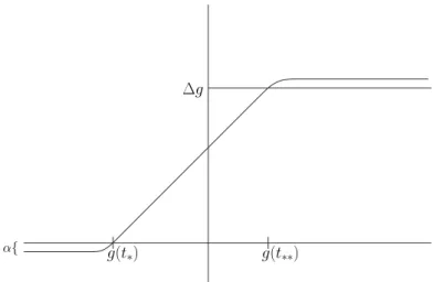
To deal honestly with the discontinuity of φ′ _{atg(t∗) and g(t∗∗), we} intro-duce a regularized function φα (cf. Figure 4) such that

φα(x) = x−g(t∗) g(t∗)≤x≤g(t∗∗), (3.18)

while at the same time

|φα|∞ ≤ osc

[tk,tk+1]

g+α, _|φ′_{α| ≤} 1.

Letting Φα :=φαΨ, (3.12) and (3.13) are satisfied, while (3.11) is replaced

by

|Φα|∞ ≤ osc

[tk,tk+1] g+α.

Repeating the calculation in (3.14) gives:

c0 osc [tk,tk+1]

g ≤ ³c0∆tk lim ε→0

Z tk+1

tk

Z 1

0

ε( ˙uε)21r(g)dx dt

´1/2

+ 1 2

µ

osc

[tk,tk+1] g+α

¶ Z tk+1

tk

dη.

Sending α to zero recovers (3.14).

α_{{ g(t}

∗∗) g(t_∗)

∆g

Figure 4: The regularized test function φα.

Lemma 3.1. Let g be inC([a, b]), h ≥0 be in L1_{([a, b]), η be a finite measure}

on [a, b], and mε ≥0 be a sequence of functions in L1([a, b]×[0,1]) with

lim

ε→0

Z tk+1

tk

Z 1

0

mεdx dt < ∞. (3.19)

Suppose that for any finite partition σ of (a, b):

σ ={a=t0 < t1 < . . . < tn =b} with ∆tk :=tk+1−tk,

we have

˜

c osc

[tk,tk+1] g _≤

µ

˜

c∆tk lim ε→0

Z tk+1

tk

Z 1

0

mεdx dt

¶1/2

+

µ

∆tk

Z tk+1

tk

h dt ¶1/2

+1

2[tkosc,tk+1] g

Z tk+1

tk

dη. (3.20)

Then

˙

g ∈L2([a, b]) (3.21)

and we have that for any δ >0,

˜

c Z b

a

( ˙g)2dt _≤ (1 +δ) lim

ε→0

Z b

a

Z 1

0

mεdx dt+

1 +δ−1

˜

c

Z b

a

Equation (3.14) is of the form (3.20) with

mε = ε( ˙uε)21r(g), ˜c = c0, h = 0.

Thus, by Lemma 3.1 we deduce:

c0

Z b

a

( ˙g)2dt ≤ (1 +δ) lim

ε→0

Z b

a

Z 1

0

ε( ˙uε)21r(g)dx dt,

and letting δ _→ 0 concludes the proof of (3.2). To see (3.3), we coarsely estimate:

c0

Z

O1

( ˙g)2dt _≤ lim

ε→0

Z

O1 Z 1

0

ε( ˙uε)21r(g)dx dt

≤ lim

ε→0

Z T

0

Z 1

0

ε( ˙uε)2dx dt

(1.34)

≤ C.¯

Letting O1 ↑ {Multg = 1} implies (3.3).

3.2

From single multiplicity to higher multiplicity

The main idea is that on sets of single multiplicity, we use Proposition 3.1, while on sets of higher multiplicity (plus a small neighborhood), we prove estimates for the Dirichlet integral of the mean:

gm :=

1

J(g1+. . .+gJ).

On the set of multiplicity J, estimates for gm give exactly the right control

since then

gm = g1 = g2 = . . . = gJ. (3.23)

To convert estimates for the mean into estimates for the interfaces, we will need the lemma:

Lemma 3.2. Suppose that g1 ≤ g2 ≤ . . . ≤ gJ are continuous functions on

[0, T]. If

˙

gj ∈L2({Mult< J}) for j = 1, . . . , J (3.24)

and

d dt

à _J

X

j=1

gj

!

∈L2(_{Mult_≤J_}), (3.25)

then

˙

In Subsection 3.3 we will show how these ingredients can be used to prove Proposition 3.2. Because the proof is somewhat technical, we first introduce the following simpler lemma. It illustrates the main idea for the case J = 2.

Lemma 3.3. Given Proposition 3.1, consider any open set O2 with

O2 ⋐ {g2(t)< g3(t)}. (3.27)

We have that

˙

gj ∈L2(O2) for j = 1,2 (3.28)

and moreover,

c0

Z

O2

( ˙g1)2+ ( ˙g2)2dt ≤ lim

ε→0

Z

O2 Z 1

0

ε( ˙uε)21r([g1, g2])dx dt. (3.29)

3.2.1 Proof of Lemma 3.3

Proof. As in the proof of Proposition 3.1, it is enough to consider the case in whichO2 is a single interval (a, b). By (3.27), we may chooser >0 sufficiently

small so that

r < 1

2 t∈inf(a,b) |g3(t)−g2(t)|.

From now on, we work entirely on [a, b] and ignoregj for j = 3. . . N.

We remark that

G2 := {g1 =g2}

is closed and [a, b]_\G2 is (relatively) open with single multiplicity. Define

Vℓ :={t;d(t, G2)<1/ℓ}, (3.30)

so that

∩∞

ℓ=1Vℓ = G2.

Let us denote the complement of a set A by Ac_{. Choose open sets U}

ℓ,1, Uℓ,2

such that

Uℓ,1 ⊃Vℓc, Uℓ,2 ⊃G2, d(Uℓ,1, Uℓ,2)≥

1

2ℓ. (3.31)

Notice in particular that

(Uℓ,1∪G2)c⊂Vℓ\G2, (3.32)

Uℓ,2\G2 ⊂Vℓ\G2 (3.33)

First, by Proposition 3.1 we have that

˙

g1,g˙2 ∈L2({Multg1 = Multg2 = 1}). (3.35)

Moreover, by (3.34), we may choose r >0 sufficiently small so that

r < 1

2 t∈infUℓ,1

|g1(t)−g2(t)|.

With this choice, the supports of 1r_(g

1) and 1r(g2) are disjoint on Uℓ,1, and

(3.2) implies the estimate

c0

Z

Uℓ,1

( ˙g1)2 + ( ˙g2)2dt

≤ lim

ε→0

Z

Uℓ,1 Z 1

0

ε( ˙uε)2(1r(g1) +1r(g2))dx dt. (3.36)

Also, we will show that gm := (g1+g2)/2 satisfies

˙

gm ∈L2(Uℓ,2) (3.37)

with the bound

2c0

Z

Uℓ,2

( ˙gm)2dt

≤ (1 +δ) lim

ε→0

Z

Uℓ,2 Z 1

0

ε( ˙uε)21r([g1, g2])dx dt+Cδ×o(1)ℓ→∞. (3.38)

Notice that (3.37) together with (3.35) implies in particular that

˙

gm ∈L2([a, b]). (3.39)

This will complete the proof, as we now explain: First, (3.35) and (3.39) imply by Lemma 3.2 that ˙g1 and ˙g2 are inL2([a, b]) which establishes (3.28). Notice

that together with (3.32) and (3.30), (3.28) implies that

Z

(Uℓ,1∪G2)c

Second, we observe:

c0

Z b

a

2

X

j=1

( ˙gj)2dt

(3.40)

≤ c0

Z

Uℓ,1

2

X

j=1

( ˙gj)2dt+c0

Z

G2

2

X

j=1

( ˙gj)2dt+o(1)ℓ→∞

(3.23)

= c0

Z

Uℓ,1

2

X

j=1

( ˙gj)2dt+ 2c0

Z

G2

( ˙gm)2dt+o(1)ℓ→∞

(3.39),(3.31)

≤ c0

Z

Uℓ,1

2

X

j=1

( ˙gj)2dt+ 2c0

Z

Uℓ,2

( ˙gm)2dt+o(1)ℓ→∞

(3.36),(3.38)

≤ lim

ε→0

Z

Uℓ,1 Z 1

0

ε( ˙uε)2(1r(g1) +1r(g2))dx dt

+(1 +δ) lim

ε→0

Z

Uℓ,2 Z 1

0

ε( ˙uε)21r([g1, g2])dx dt+Cδ×o(1)ℓ→∞

≤ (1 +δ) lim

ε→0

Z b

a

Z 1

0

ε( ˙uε)21r([g1, g2])dx dt+Cδ×o(1)ℓ→∞. (3.41)

Sending first ℓ→ ∞ and then δ→0 completes the proof of (3.29). Thus, we need only show (3.37) and (3.38).

As usual, it suffices to consider the case that Uℓ,2 is a single interval (c, d).

Letσ be an arbitrary, finite partition of (c, d):

σ=_{c=t0 < t1 < . . . < tn=d} with ∆tk :=tk+1−tk.

Case 1: [tk, tk+1] ∩ G2 = ∅. Then by Proposition 3.1, ˙g1 and ˙g2 are

L2_([t

k, tk+1]) and

2c0 osc (tk,tk+1)

gm ≤ c0

µ

osc

(tk,tk+1)

g1+ osc (tk,tk+1)

g2

¶

≤ c0

µZ tk+1

tk

|g˙1|+|g˙2|dt

¶

≤ √2c0

µ

∆tk

Z tk+1

tk

( ˙g1)2+ ( ˙g2)2dt

¶1/2

, (3.42)

the last line following from H¨older’s inequality and the inequality

√

Case 2: [tk, tk+1]∩G2 6=∅. All operations below (argmin, infimum, etc...)

are over the interval [tk, tk+1], and for ease of notation, we omit writing the

interval. In analogy with the proof of Proposition 3.1, we define

t∗ := argmingm, t∗∗:= argmaxgm, (3.43)

and assume without loss that t∗ < t∗∗. We would like to build a test function Φ(x, t) such that

Z 1

0

Φ(x, t)dµt = c0

³

Φ(g1(t), t) + Φ(g2(t), t)

´

∀t∈(a, b), (3.44)

Φ(g2(t∗∗)) + Φ(g1(t∗∗))−

³

Φ(g2(t∗)) + Φ(g1(t∗))

´

= 2 oscgm, (3.45)

while at the same time, the following properties hold:

|Φ_|∞ ≤ supg2−infg1

lim

ε→0

Z t∗∗

t∗ Z 1

0

˙Φ³ε 2(uε,x)

2_+ε−1_W(u

ε)

´

dx dt = 0,

lim

ε→0

Z tk+1

tk

Z 1

0 |

Φxεuε,xu˙ε|dx dt

≤ µ

2c0∆tk lim ε→0

Z tk+1

tk

Z 1

0

ε( ˙uε)21r([g1, g2])dx dt

¶1/2 .

(3.46)

Given such a test function, we calculate (similarly to in (1.33) or (3.14)):

2c0oscgm

(3.44)(3.45)

=

Z 1

0

Φdµt∗∗ − Z 1

0

Φdµt∗

= lim

ε→0

Z t∗∗

t∗

d dt

Z 1

0

Φ³ε 2(uε,x)

2_+ε−1_W(u

ε)

´ dx dt

(3.46)

≤ ³2c0∆tk lim ε→0

Z tk+1

tk

Z 1

0

ε( ˙uε)21r([g1, g2])dx dt

´1/2

+1

2(supg2−infg1)

Z tk+1

tk

dη. (3.47)

The idea for the test function is

Φ(x, t) = φ(x)Ψ(x, t),

where now φ is the function

φ(x) =

  

 

infg1−infgm x <infg1

x₋infgm infg1 ≤x≤supg2