超対称ランダウ・ギンツブルグ模型の赤外臨界点の数値的研究

(1)

九州大学学術情報リポジトリ

Kyushu University Institutional Repository

超対称ランダウ・ギンツブルグ模型の赤外臨界点の数値的研究

森川, 億人

http://hdl.handle.net/2324/4474929

出版情報：Kyushu University, 2020, 博士（理学）, 課程博士バージョン：

権利関係：

(2)

Ph.D. Thesis

Numerical study of infrared criticality of the supersymmetric Landau–Ginzburg model

超対称ランダウ・ギンツブルグ模型の赤外臨界点の数値的研究

Okuto Morikawa

Department of Physics, Kyushu University, 744 Motooka, Nishi-ku, Fukuoka, 819-0395, Japan

December 20, 2020

(3)

(4)

Abstract

In sufficiently low energies, that is, at the infrared (IR) fixed point, quantum field theories are expected to be scale invariant. Such a scale-invariant theory would be described by a conformal field theory (CFT). If a quantum field theory gives rise to a nontrivial CFT at the IR fixed point, the original theory is called the Landau–Ginzburg (LG) description of the CFT, or the LG model. In particular, as an example of the supersymmetric LG model, it is believed that the two-dimensional N = (2,2) Wess–Zumino (2D N = 2 WZ) model corresponds to the 2DN = 2 superconformal field theory (SCFT). This conjecture of the LG description has been theoretically analyzed from various aspects. It is, however, difficult to prove this theoretical conjecture directly, since the coupling constant becomes strong at the IR region. Moreover, because this is the lower-dimensional massless system, the perturbation theory possesses severe IR divergences. For these reasons, the LG description is a remarkable non-perturbative phenomenon.

This issue is closely related to superstring theory. Superstring theory is expected to describe quantum gravity, and provide a candidate for a theory of everything, which unifies all fundamental forces. In superstring theory, we observe a four-dimensional spacetime, while there exists an extra six-dimensional space, which is compactified into the Calabi–Yau (CY) manifold. Then, scattering amplitudes in a superstring theory with the CY compactification can be computed from an N = 2 SCFT, by which the world sheet theory is described.

However to pursue this strategy is quite difficult because such a SCFT is in general not a solvable minimal model. Thus, it is hard to carry out any computation for a general CY manifold and to treat phenomena relating to the dynamics of spacetime. The LG description, on the other hand, realizes a strongly-interacting Lagrangian with the superpotential corresponding to the geometry of the CY manifold; we can deform the geometry of the superstring compactification by manipulating the superpotential. Therefore, if we can analyze such a strongly-interacting field theory directly, the study of the LG model would be a new approach to look into superstring theory.

An useful approach to this issue may be provided by a non-perturbative calculational method such as the lattice field theory. A quantum field theory is defined as a discretized theory on a spacetime lattice. Implementation of such a lattice formulation on the computer enables us to calculate physical quantities from first principles. As is well recognized, however, the spacetime lattice is generally incompatible with spacetime symmetries such as the supersymmetry (SUSY). Although those symmetries are expected to restore in the continuum limit, this is an obstacle to the lattice study on supersymmetric field theories. Despite this difficulty, there are some recent numerical studies for the WZ model with the cubic superpotential; the scaling dimension and the central charge in the correspondingA2 minimal model were measured. These numerical studies achieved a triumph of the lattice field theory, and

i

(5)

ii

provides a non-perturbative evidence of the WZ/minimal-model correspondence.

In this thesis, we numerically study the 2D N = 2 WZ model, by using the formulation by Kamata and Suzuki. This formulation is based on the Nicolai map and the momentum cutoff regularization; allowing the action to be non-local, the theory preserves the full set of SUSY even with a finite cutoff, as well as the translational invariance. We focus on the following three numerical studies: (A) the numerical simulation of the ADE-type theories and verification of the theoretical conjecture; (B) the continuum limit analysis of the scaling dimension based on the finite-size scaling; (C) the application to the torus compactification of superstring theory.

(A) We apply the SUSY-preserving formulation to the following various ADE-type theories: the A2, A3, D3, D4, E6 (∼= A2 ⊗A3), and E7 models. In some aspects, we extend and improve the theoretical and numerical analyses in the preceding works. First, to study theDE minimal models and further applications, the method is generalized to one with multiple superfields and more complicated superpotentials. Second, for the A2 minimal model, numerical accuracy is quite improved. Third, we numerically measure the scaling dimension, by using the two-point function of the scalar field in the momentum space. Also we numerically measure the central charge, by using the two-point function of the supercurrent and that of the energy-momentum tensor. Our results are consistent with the conjectured WZ/minimal-model correspondence.

(B) We develop an extrapolation method to take the continuum and infinite-volume limit, while any extrapolation has been not done in the preceding numerical studies. Then, we perform a precision measurement of the scaling dimension in theA₂-type theory. This result implies the restoration of the locality in the continuum limit.

(C) We apply the above method to non-minimal SCFTs. For simplicity we consider the complex one-dimensional torus compactification. This theory may be simply described by theA2⊗A2⊗A2 minimal model. To deform the geometry of the compactification, we add a would-be marginal operator to the superpotential; then, the central charge is believed not to depend on this deformation. We numerically observe the central charge being constant under this deformation, which provides the non-perturbative evidence of the conjecture.

These studies show a coherence picture which is consistent with the conjecture of the LG description of SCFT, and support the validity of our formulation. This kind of numerical approach, when further developed, will come in useful to study superstring theory.

This thesis is based on the following papers:

• O. Morikawa and H. Suzuki,

“Numerical study of the N = 2 Landau–Ginzburg model,”

PTEP 2018no.8, (2018) 083B05,arXiv:1805.10735 [hep-lat].

• O. Morikawa,

“Numerical study of the N = 2 Landau–Ginzburg model with two superfields,”

JHEP 12(2018) 045,arXiv:1810.02519 [hep-lat].

• O. Morikawa,

“Continuum limit in numerical simulations of the N = 2 Landau–Ginzburg model,”

PTEP 2019no.10, (2019) 103B03,arXiv:1906.00653 [hep-lat].

(6)

List of Figures

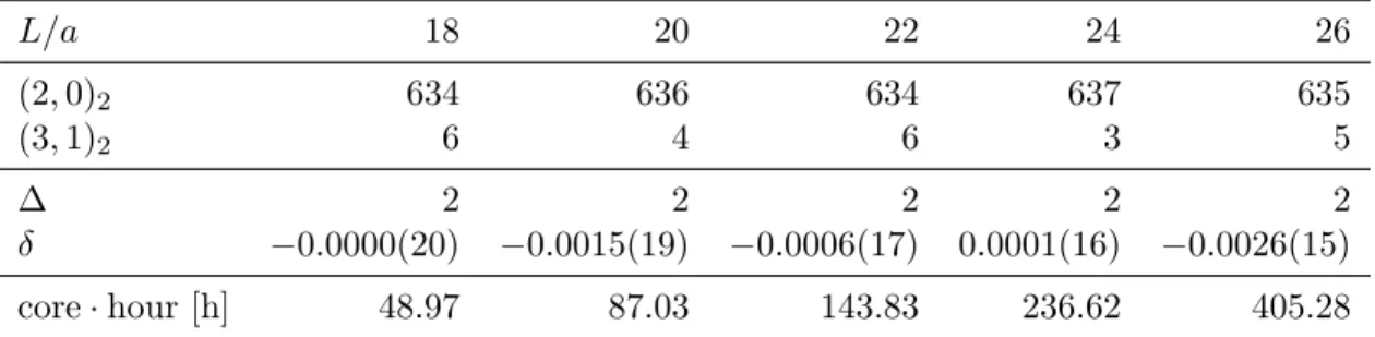
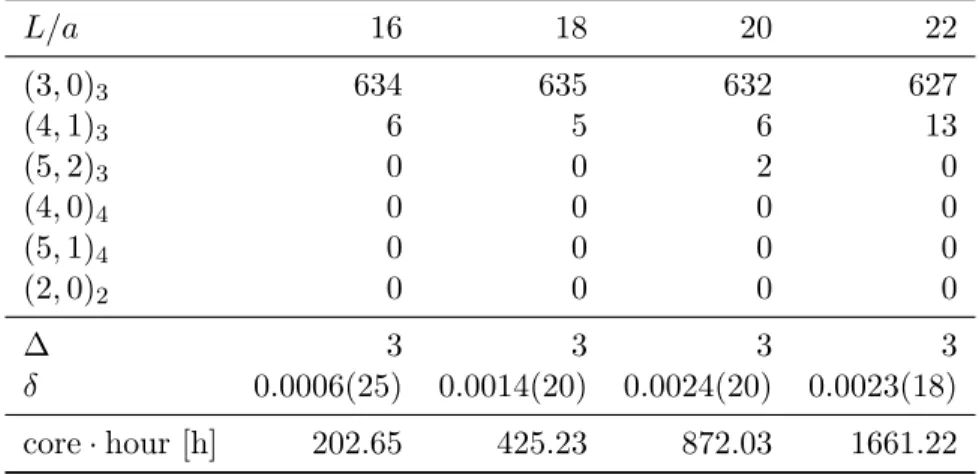
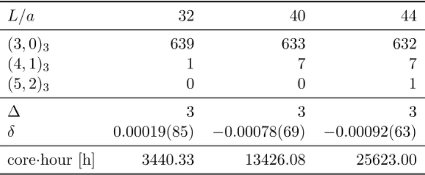
5.1 Computational time as a function of the lattice size. . . 46

5.2 SUSY WT relation of Eq. (5.32) forA₂,L/a= 36, and ap₁ =π. . . 48

5.3 SUSY WT relation of Eq. (5.32) forA₂,L/a= 36, and ap₁ =π/18. . . 48

5.4 SUSY WT relation of Eq. (5.32) forA3,L/a= 30, and ap1 =π. . . 49

5.5 SUSY WT relation of Eq. (5.32) forA₃,L/a= 30, and ap₁ =π/15. . . 49

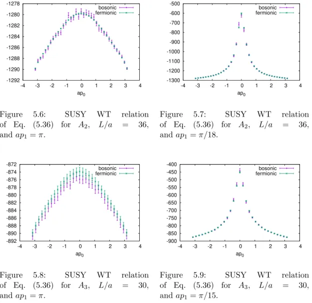
5.6 SUSY WT relation of Eq. (5.36) forA₂,L/a= 36, and ap₁ =π. . . 50

5.7 SUSY WT relation of Eq. (5.36) forA2,L/a= 36, and ap1 =π/18. . . 50

5.8 SUSY WT relation of Eq. (5.36) forA₃,L/a= 30, and ap₁ =π. . . 50

5.9 SUSY WT relation of Eq. (5.36) forA₃,L/a= 30, and ap₁ =π/15. . . 50

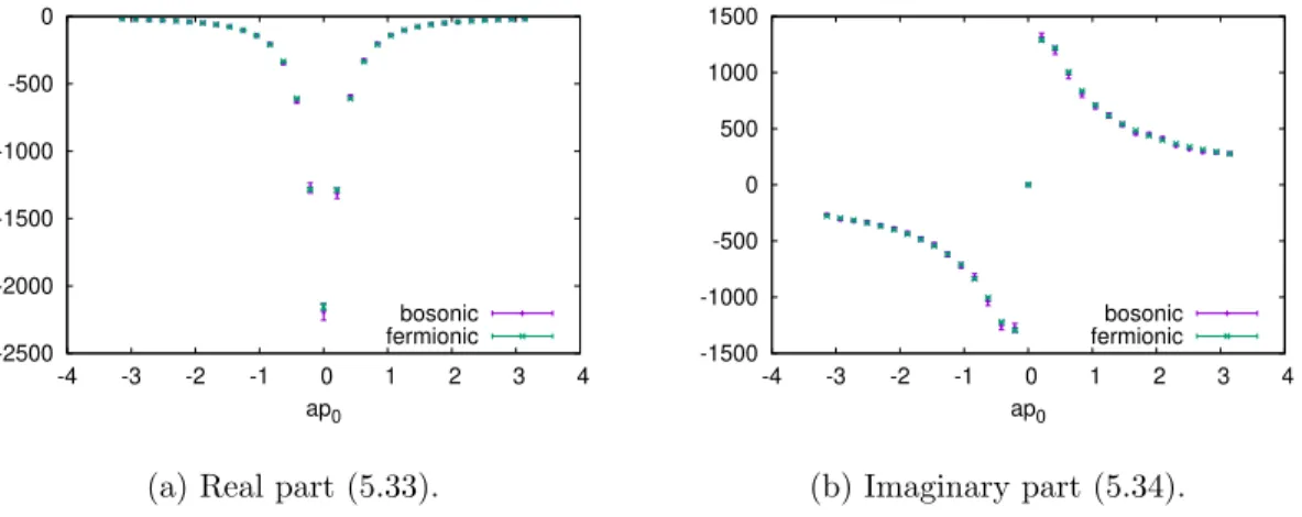
5.10 SUSY WT relation of Eq. (5.33) forA2,L/a= 8 and ap1=π. . . 51

5.11 SUSY WT relation of Eq. (5.36) forA₂,L/a= 8 and ap₁=π. . . 51

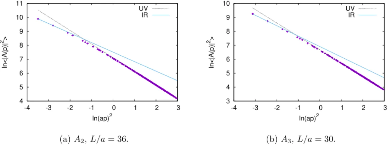
6.1 lnhA(p)A^∗(−p)i as a function of ln(ap)²forA₂ andA₃. The broken and solid lines are linear fits in the UV and IR regions, respectively. . . 54

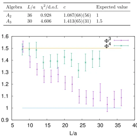
6.2 Scaling dimensions obtained for A₂ andA₃ with various box sizes. . . 55

6.3 Scaling dimensions obtained for A2 and A3 from the linear fitting in various momentum regions from IR to UV, ^2π_Ln≤ |p|< ^2π_L(n+ 1), for n∈Z⁺. . . 56

6.4 hS⁺(p)S⁻(−p)iforA2,L/a= 36, andap1 =π/18. The fitting curves from Eq. (6.17) are also depicted. . . 58

6.5 hS⁺(p)S⁻(−p)iforA3,L/a= 30, andap1 =π/15. The fitting curves from Eq. (6.17) are also depicted. . . 58

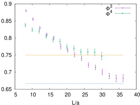
6.6 Central charges obtained by the fit for A2 (W = Φ³) and A3 (W = Φ⁴) as a function of the box sizeL/a= 8–36. . . 59

6.7 “Effective central charge” obtained by the fit forA2 andA3 in various momentum regions, ^2π_Ln≤ |p|< ^2π_L(n+ 1) (n= 1, . . . , L−1). . . 60

6.8 hT(p)T(−p)i forA2,L/a= 36, and ap1=π/18. The fitting curve of Eq. (6.22) is also depicted. . . 61

6.9 hT(p)T(−p)iforA3,L/a= 36, andap1 =π/15. The fitting curve by Eq. (6.22) is also depicted. . . 61

6.10 Central charges obtained by the fit for A2 (W = Φ³) and A3 (W = Φ⁴) as a function of the box sizeL/a= 8–36. . . 62

6.11 “Effective central charge” obtained by the fit forA2 andA3 in various momentum regions, ^2π_Ln≤ |p|< ^2π_L(n+ 1) (n∈Z+). . . 63

6.12 hT(p)T(−p)i for D3, L/a = 44, and ap1 = π/22. The fitting curve (6.22) is depicted at once. . . 64

v

(9)

vi LIST OF FIGURES 6.13 hT(p)T(−p)i for D4, L/a = 42, and ap1 = π/21. The fitting curve (6.22) is

depicted at once. . . 64 6.14 hT(p)T(−p)i for E₇, L/a = 24, and ap₁ = π/12. The fitting curve (6.22) is

depicted at once. . . 65 6.15 Systematic error estimation for the central charge forD3,D4,E7. . . 66 6.16 “Effective central charge” for D₃, D₄, and E₇, which changes as the function

of |p|= ^2π_Lnwith fitted momentum regions, ^2π_Ln≤ |p|< ^2π_L(n+ 1), for n∈Z+. . . 67 6.17 Σ(u, a/L)-(a/L) plot withu= 3.9175. The fitting line of Eq. (6.40) is also depicted. 72 6.18 ˜Σ(u, a/L)-(a/L) plot withu= 3.9175. The fitting curve of Eq. (6.48) is also depicted. 75

(10)

List of Tables

2.1 Infinitesimal conformal transformation in d-dimensional Euclidean space (d >2) . 8

4.1 ADE classification . . . 34

5.1 Classification of configurations for A2 (W = Φ³). . . 43

5.2 Classification of configurations for A₂ (W = Φ³) (continued). . . 43

5.3 Classification of configurations for A2 (W = Φ³) (continued). . . 43

5.4 Classification of configurations for A₃ (W = Φ⁴). . . 43

5.5 Classification of configurations for A₃ (W = Φ⁴) (continued). . . 44

5.6 Classification of configurations for A3 (W = Φ⁴) (continued). . . 44

5.7 Classification of configurations for D₃. . . 44

5.8 Classification of configurations for D3 (continued). . . 45

5.9 Classification of configurations for D4. . . 45

5.10 Classification of configurations forD₄ (continued). . . 45

5.11 Classification of configurations forE7. . . 46

6.1 Scaling dimensions obtained forA₂andA₃ from the linear fit in the IR region ^2π_L ≤ |p|< ^4π_L. . . 54

6.2 The central charges for A2 and A3 obtained from the fit of the supercurrent correlator. The fitting momentum region is ^2π_L ≤ |p|< ^4π_L. . . 59

6.3 The central charges for A₂ and A₃ obtained from the fit of the EMT correlator. The fitting momentum region is ^2π_L ≤ |p|< ^4π_L. . . 60

6.4 The central charge forD₃,D₄ andE₇ obtained from the fit of the EMT correlator. The fitted momentum range is ^2π_L ≤ |p|< ^4π_L. . . 65

6.5 Classification of the configurations obtained for theA2-type theory with tunedλ. . 70

6.6 Quality of the configurations obtained for theA₂-type theory with tunedλ. . . 71

6.7 Scalar susceptibility with u= 3.9175. . . 71

6.8 Scaling dimension measured at finite volumes. The results in the last two rows are obtained by reading the slope of lnχ for (L/a, L⁰/a) = (24,48) or (L/a, L⁰/a) = (26,52) in Table 6.7. . . 71

6.9 lnχ(L⁰) with u= 3.9175 andL/a= 52 when the number of configurations,N_conf, varies. . . 73

6.10 Classification of configurations for Eq. (6.51) withβ = 0.1 . . . 76

6.11 Classification of configurations for Eq. (6.51) withβ = 1 . . . 76

6.12 Classification of configurations for Eq. (6.51) withβ = 10 . . . 77

6.13 The scaling dimension obtained from the fit ofhA₁A1ifor Eq. (6.51) with various values of β. The fitted momentum range is ^2π_L ≤ |p|< ^4π_L. . . 78

vii

(11)

viii LIST OF TABLES 6.14 The scaling dimension obtained from the fit ofhA₂A2ifor Eq. (6.51) with various

values of β. The fitted momentum range is ^2π_L ≤ |p|< ^4π_L. . . 78 6.15 The scaling dimension obtained from the fit ofhA₃A₃ifor Eq. (6.51) with various

values of β. The fitted momentum range is ^2π_L ≤ |p|< ^4π_L. . . 78 6.16 The central charge obtained from the fit of the EMT correlator for Eq. (6.51) with

various values of β. The fitted momentum range is ^2π_L ≤ |p|< ^4π_L. . . 79 7.1 The scaling dimensions and the central charges obtained. . . 81

(12)

Acknowledgements

First of all, I would like to show my profound gratitude to my supervisor, Prof. Hiroshi Suzuki, for his continuous supports. He always encouraged me on my research since I was an under- graduate student. He suggested a lot of interesting and exciting topics to study, and was willing to provide valuable feedback on them. From his insightful comments and the ex- tensive discussions with him, I learned various ideas on physics and sincere attitudes as a researcher.

I am grateful to Prof. Koji Harada, Prof. Takashi Hara, and Prof. Yoshifumi R. Shimizu, for their valuable advice. They also supported my research as the advisory committee.

I would like to extend my thanks to Prof. Koji Tsumura, Prof. Ken-ichi Okumura, and Prof. Takuma Matsumoto, for their kind words and the wide-ranging discussions.

I would like to express my appreciation to Prof. Hisao Suzuzki for giving me various ideas about applications of my research to superstring theory, Prof. Hiroto So and Prof. Noboru Kawamoto for instructing me in supersymmetry on the lattice. I was encouraged by their comments and useful discussions with them. I show my gratitude to Dr. Issaku Kanamori, Dr. Daisuke Kadoh, Dr. Akio Tomiya, and Dr. Katsumasa Nakayama for meaningful discussions on the lattice simulation. My gratefulness would go to the members of WHOT-QCD Collaboration for their hospitality.

I was supported other members in Theory of Elementary Particles Laboratory; and other people in Theoretical Nuclear Physics Laboratory and Theory of Subatomic Physics and Astrophysics Laboratory. I especially would like to express my thanks to my three seniors:

Dr. Hiromasa Takaura, Dr. Aya Kasai, and Mr. Hiroki Makino. They kindly taught me many aspects of physics about which I had dubious ideas. They are also the collaborators on my project, and have sophisticated skills based on a deep physical viewpoint, which was very helpful in my research. My thanks also go to Dr. Masahiro Ishii, Dr. Junpei Sugano, Dr. Takehiro Hirakida, Mr. Kenji Hieda, Mr. Shoya Ogawa, and Mr. Yushin Yamada, for their fruitful comments in casual conversation.

I show my appreciation to Ms. Yuki Yamaji, Ms. Megumi Ieda, Ms. Atsuko Sono, Ms.

Mayumi Takaki, Ms. Mariko Ishii, Ms. Mariko Komiya, and Ms. Mako Nagata for their practical supports.

The numerical computations in this thesis were partially carried out by supercomputer system ITO of Research Institute for Information Technology (RIIT) at Kyushu University.

The work was supported by Grant-in-Aid for Scientific Research (KAKENHI) Grant Number JP18J20935 from the Japan Society for the Promotion of Science (JSPS).

ix

(13)

(14)

Chapter 1

Introduction

1.1 Landau–Ginzburg description of the conformal field theory

The dynamics of elementary particles is described by a theoretical framework, quantum field theory. Its microscopic structure at short distances or in high energies effects long-distance or low-energy physics in a complicated way because of quantum radiations. An effective way to analyze this has been developed by renormalization group (RG) transformation [1]. The flow of RG transformations, which is called the RG flow, governs the behavior of a quantum field theory under some rigid scale transformations, which act as the “coarse-graining” between different scales.

In an extremely low-energy scale, that is, at the infrared (IR) fixed point of the RG flow, any quantum field theory is expected to possess the scale invariance, while all massive modes are decoupled. Such a scale-invariant theory would be described by a conformal field theory (CFT) [2]. If a quantum field theory gives rise to a nontrivial CFT at the IR fixed point, the original field theory is called the Landau–Ginzburg (LG) description of the CFT [3], or the LG model. The LG description thus provides a Lagrangian-level realization of CFT, and is characterized by a nontrivial critical behavior under the RG flow. Originally, this idea of the LG model was introduced as a phenomenological model to describe superconductivity [4]; in this context, we use the free energy instead of the Lagrangian. Such critical phenomena are of great interest in a wide range of physics.

Although the existence of such a Lagrangian is not always obvious, if we know it, tech- niques developed in quantum field theory provide a quite important tool to clarify conformally invariant systems. As another famous example, the Feigin–Fuks (integral) representation [5,6]

gives a free-field Lagrangian on curved spacetime. Feigin and Fuks employed this to explore the unitary representation of the Virasoro algebra, and proved the Kac determinant formula in an elegant way (see Chap. 2). Analyses of the Lagrangian such as their technique have come in useful [7, 8] for performing many computations explicitly and understanding the systems intuitively.

It is also important to consider the fermionic extension of the conformal symmetry by the supersymmetry (SUSY) [9–11], which is a symmetry under swapping bosons and fermions.

This extended symmetry, superconformal symmetry, is realized in the two-dimensional (2D) world sheet theory of superstring theory, which is expected to describe quantum gravity [12–

1

(15)

2 CHAPTER 1. INTRODUCTION 14], and provide a candidate for a theory of everything unifying all fundamental forces.¹ In superstring theory, because of the consistency of the theory, we observe a four-dimensional spacetime, while there exists an extra six-dimensional space [17–23]. Requiring the SUSY on the four-dimensional spacetime, the extra dimensions are considered to be compactified into the Calabi–Yau (CY) manifold [24, 25]. Then, we have a 2DN = 2 superconformal field theory (SCFT) on the world sheet.² Scattering amplitudes in a superstring theory with the CY compactification can be computed from this SCFT. We can pursue this strategy if such a SCFT is a solvable minimal model or a tensor product of minimal models (Gepner model [26, 27]), but it is in general not the case. Thus, it is hard to carry out any computation for a general CY manifold, and treat phenomena which relate to the dynamics of the compactification.

Now, an alternative approach may be provided by the LG description of SCFT, while a 2D N = 2 LG model becomes a N = 2 SCFT at infrared criticality. It is believed [26–37]

that an example of this is given by the 2DN = 2 massless Wess–Zumino (WZ) model with a quasi-homogeneous superpotential, which can be obtained by the dimensional reduction of the four-dimensional WZ model [38]. It is known that the structure of the superpotential is closely related to the geometry of the CY manifold [39–42]. One can easily change the superpotential, which causes the deformation of the geometry of the superstring compactification.

The above theoretical conjecture of the LG description has been studied from various aspects, which support this correspondence [39, 43–52]. For example, Refs. [43, 46, 48] argue the RG flow for the WZ model with the monomial superpotential, W(Φ) ∝ Φⁿ⁺¹, which corresponds to the A_n minimal model of the N = 2 SCFT; the correspondence between the superpotential and the ADE minimal model is classified in Ref. [44]. See Refs. [53, 54] for reviews. It is, however, difficult to prove this theoretical conjecture directly, since the 2D N = 2 massless WZ model is strongly coupled at low energies. Moreover, because this is the lower-dimensional massless system, the perturbation theory suffers from IR divergences. The LG description is thus truly a non-perturbative phenomenon.

1.2 Lattice field theory and the numerical approaches

A non-perturbative calculational method may be provided by the lattice field theory [55].

The lattice field theory is the most well-developed framework to study non-perturbative phenomena in quantum field theories; it provides the lattice regularization that the continuum spacetime is discretized as the set of points called the lattice. Then, a quantum field theory is defined as a discretized theory on the spacetime lattice with finite degrees of freedom. Imple- mentation of such a formulation on the lattice (lattice formulation) on a computer enables us to calculate physical quantities of interest from first principles. As is well recognized, however, the lattice formulation is in general not compatible with the SUSY, because the SUSY is one of spacetime symmetries; schematically

{Q,Q} ∼¯ ∂, (1.1)

where Q ( ¯Q) is the charge associated with the SUSY (supercharge), and the derivative ∂ denotes the translation. (We will discuss this anti-commutation relation in Chap. 3.) While

1The original string theory was considered as a theory of hadrons mainly from 1968 to 1975. For these studies, see Ref. [15] for a review. For developments in 1980s, Ref. [16] gives a detailed review.

2Here, we consider the 2DN = (2,2) supersymmetry, and notN = (2,0). For more details, see Chap. 3.

(16)

1.3. NUMERICAL STUDY OF THE2DN = 2 WZ MODEL 3 the SUSY must be a crucial element to study the above LG description, as a usual way, lattice parameters should be fine-tuned so that the lattice formulation yields the target SUSY- invariant theory in the continuum limit; this fact complicates actual numerical studies [56–

59].³

Despite this difficulty, recently, the authors of Ref. [61] studied the case of a cubic superpo- tentialW = Φ³, which is considered to correspond theA2 minimal model; they measured the scaling dimension of the scalar field in the IR limit by using a lattice formulation of Ref. [62].⁴ In Ref. [61], one can observe good agreement of the scaling dimension with that of the A2

minimal model. The formulation of Ref. [62] exactly preserves one nilpotent SUSY at finite lattice spacing (not full SUSY)⁵, and the vacuum energy is canceled even on the lattice thanks to the existence of the so-called Nicolai or Nicolai–Parisi–Sourlas map [69–72]. Because of this preserved SUSY, and since this lower-dimensional theory is super-renormalizable, it can be argued, to all orders of perturbation theory, that the full set of the SUSY is automatically restored in the continuum limit [73, 74]. The study of Ref. [61] thus achieved a triumph of the lattice field theory, and paved the way for the numerical investigation of the LG model.

Somewhat later, the authors of Ref. [75] examined the same A2-type WZ model with a cubic superpotential by using the formulation from Ref. [76]; they measured not only the scaling dimension but also the central charge. The formulation in Ref. [76] is based on the Nicolai map and a momentum cutoff regularization. A remarkable feature is that the formulation preserves the full SUSY as well as the translational invariance even with a finite cutoff. Owing to this fact, it is straightforward to construct the Noether current associated with spacetime symmetries, for instance the supercurrent for the SUSY.⁶ Then, from the numerical simulation of the two-point function of the supercurrent, the central charge was observed, which is fairly consistent with theA₂ minimal model.

The latter formulation is (almost) identical to the dimensional reduction of the lattice formulation [77] of the 4D N = 1 WZ model on the basis of the SLAC derivative [78, 79].

Although this formulation exactly preserves SUSY, it is well recognized that it breaks the locality because of the SLAC derivative. For the 2D massive N = 2 WZ model, because of the exactly preserved SUSY and because this theory is super-renormalizable, it can be argued [76], to all orders of perturbation theory, that the locality is automatically restored in the continuum limit. Although, strictly speaking, the theoretical basis of the formulation for the massless WZ model is not obvious, the above numerical results support the validity of the formulation, and the restoration of the locality. This is an interesting observation left as a future problem.

1.3 Numerical study of the 2D N = 2 WZ model

In this thesis, following on from the study of Ref. [75], we numerical study the 2DN = 2 WZ model by employing the SUSY-invariant formulation of Ref. [76]. We extend and improve the

3Ref. [60] is a recent review of the SUSY on the lattice, which refers to lattice formulations of the 2DN = 2 WZ model.

4References [63–67] are preceding studies on the 2D massiveN = 2 WZ model.

5This feature is common to the lattice formulation studied in Ref. [68].

6In a lattice formulation such as that in Ref. [61,62], the explicit expression of the Noether current associated with spacetime symmetries is quite nontrivial because the regularization breaks such symmetries and the Noether’s theorem cannot work well.

(17)

4 CHAPTER 1. INTRODUCTION theoretical and numerical analyses in Ref. [75] in several aspects.

To obtain further support for the conjectured LG correspondence and the validity of the formulation, we study the following higher critical models: theA3,D3,D4,E6∼=A2⊗A3,E7

models, as well as theA₂ model [80, 81]. First, the method in Ref. [75] is then generalized to the WZ model with multiple superfields and more complicated superpotentials. Second, the numerical accuracy and the effective number of configurations in the Monte Carlo simulation are quite improved. Third, for the scaling dimension, we use the two-point function of the scalar field in the momentum space instead of the susceptibility of Ref. [75]. We also measure the central charge by using the two-point function not only of the supercurrent but also of the energy–momentum tensor (EMT). In Ref. [75], it was found that the EMT correlation function was too noisy to extract the central charge; in this thesis, we settle this problem by using SUSY Ward–Takahashi relations. It turns out that our prescription for the correlation function of the EMT is rather useful to measure the central charge. We also calculate the “effective central charge” as in Ref. [75] that is an analogue of the ZamolodchikovC-function [82, 83].

All these results for typicalADE-type theories show a coherence picture, which is consistent with the conjectured WZ/minimal-model correspondence.

In this thesis, we also consider an extrapolation method to take the continuum limit [84].

Although the SCFT is defined as the continuum theory with the infinite volume, the results of the preceding works and ours above are not extrapolated to the continuum/infinite-volume limits. Moreover, one can find that the computation of the scaling dimension in Ref. [75] is quite sensitive to a ultraviolet (UV) ambiguity because of the locality breaking. To justify numerical studies based on the formulation, it should be observed that such a UV ambiguity disappear in the continuum/infinite-volume limit. We develop the finite-size scaling analysis in Refs. [61, 75] into a continuum-limit extrapolation method. The extrapolation also carries out the infinite volume limit. We then apply this extrapolation method to the above numerical approach. We study the A2-type WZ model with the cubic superpotential, and perform a precision measurement of the scaling dimension by using this extrapolation method. This is a more reliable result, and is rather consistent with the conjecturedA₂-type correspondence.

Finally, we apply the present numerical approach to the SCFT which is not a minimal model. For simplicity the complex one-dimensional torus compactification is studied. In a simple way, this theory is described by the Gepner model,A₂⊗A₂⊗A₂, which corresponds to the superpotential of the formx³+y³+z³. If we add a term xyz to the superpotential, which does not correspond a Gepner model but is still quasi-homogeneous, the geometry of the compactification is deformed. This term xyz is believed to be a marginal operator, and so the central charge would not depend on this deformation. As mentioned above, however it is difficult to treat such deformations in the compactification in usual analyses of superstring theory; this is an interesting non-perturbative problem. We numerically simulate the WZ model with this superpotential, while the deformation parameter is varied; the central charge is directly measured. From our result we see the central charge being constant under this deformation, which provides the non-perturbative evidence of the conjecture.

All these studies are consistent with the theoretical conjecture of the LG/SCFT correspondence, and support the validity of the formulation of Ref. [76]. In view of the LG/CY correspondence [39–42], we hope that this kind of numerical method, when further developed, will eventually provide a computation method for scattering amplitudes in a superstring theory, whose world sheet theory is not necessarily a Gepner model.

(18)

1.4. ORGANIZATION OF THE THESIS 5

1.4 Organization of the thesis

This thesis is organized as follows: In Chap. 2, we give a review of 2D CFT to introduce the necessary ideas we will use later. We also review the SUSY and the superconformal symmetry in Chap. 3, by using explicit computations in the 2D WZ model. Especially, we derive the explicit form of the important Noether currents: the supercurrent, the EMT, and the U(1) current; we show that those currents form the superconformal multiplet in the massless free WZ model. In Chap. 4, we discuss the RG, and the LG description of CFT together with the LG/CY correspondence. We then introduce the Zamolodchikov’s c- theorem and its SUSY-analogue. In Chap. 5, we examine the SUSY-invariant formulation studied in Ref. [76]. To provide consistency checks of the simulation based on this, we show that the Witten index and some SUSY WT relations are reproduced. Chapter 6 is the main part of this thesis; we investigate the WZ model at IR criticality and give our numerical results. In the first two sections, we focus on theADE-type WZ model, which corresponds to the minimal model of SCFT. We measure the scaling dimension from the scalar correlator and the central charge from the two-point functions of the above Noether currents. In Sect. 6.3, we develop the continuum-limit analysis, and perform precision measurement of the scaling dimension. Finally, in Sect. 6.4, we measure the central charge under the deformation of the torus compactification. Chapter 7 is devoted to the conclusions. In Appendix A, we present a fast algorithm for the practical numerical computation.

(19)

(20)

Chapter 2

Conformal field theory

2.1 Conformal transformation

Let us briefly introduce basic ideas of the conformal field theory (CFT) [2]. The most part in this chapter is based on the discussion in Ref. [53, 85]. In what follows, in d-dimensions, Green indices,µ,ν, . . . run over 0, 1, . . . ,d−1; repeated indices are not summed over.

If for manifoldsM andM⁰ a differentiable mappingϕ:M →M⁰ is a one-to-one mapping and the inverse ϕ⁻¹ is differentiable, then ϕ is called a diffeomorphism. Given a Riemann metric ds²=P

µ,νgµν(x)dx^µdx^ν on the manifold M, a diffeomorphism fromM toM

gµν(x)→g_µν⁰ (x⁰) =e^ω(x)gµν(x) (2.1) is known as a conformal transformation, where ω(x) is an arbitrary real function. The set of all conformal transformations forms the conformal group. As usual, a Killing vectorv^µ is given as an infinitesimal generator of the isometry group, such that the metric is invariant

δgµν(x) = 0 (2.2)

under an infinitesimal transformation x^µ → x^µ+δx^µ = x^µ+v^µ(x). Now, from Eq. (2.1), let us consider an infinitesimal coordinate transformation, under which the mapped Riemann metric isconformally equivalent to the original one:

δgµν(x)∝gµν(x). (2.3)

In other words, the metric is invariant under a coordinate transformationx^µ→ x^µ+v^µ(x) and a local rescaling of the metric known as the Weyl transformation [86, 87]

g_µν(x)→g⁰_µν(x) =e^ω(x)g_µν(x). (2.4) Then,v^µis called a conformal Killing vector, and is an infinitesimal generator of the conformal group.

If a field theory has the conformal symmetry, which is a invariance under conformal transformations, the theory is called a conformal field theory. Since any conformal transformation induces the Weyl transformation, conformal field theories on curved spacetime is invariant under Weyl transformations; this is the Weyl symmetry.

7

(21)

8 CHAPTER 2. CONFORMAL FIELD THEORY v^µ

translation a^µ

rotation P

νω^µ_νx^ν (ω_µν =−ω_νµ) scaling transformation (dilatation) λx^µ

special conformal transformation |x|²b^µ−2(b·x)x^µ

Table 2.1: Infinitesimal conformal transformation in d-dimensional Euclidean space (d >2) In the d-dimensional Euclidean space, we obtain the conformal Killing equation as

∂_µv_ν(x) +∂_νv_µ(x) = 2 d

X

ρ

∂_ρv^ρ(x)δ_µν. (2.5)

Table 2.1 shows the set of the Killing vectors in the d-dimensional Euclidean spacetime with d > 2. We note that, for d > 2, there exists a finite number of generators. On the other hand, if we setd= 2, the conformal Killing equation reduces to

∂v¯ ^z = 0, (2.6)

where we have introduced the complex coordinatez=x⁰+ix¹, and

v^z≡v⁰+iv¹, v^z^¯≡v⁰−iv¹, (2.7)

∂≡ ∂

∂z = 1

2(∂0−i∂1), ∂¯≡ ∂

∂z¯= 1

2(∂0+i∂1). (2.8) Thereforev^z is a holomorphic function, and v^z^¯ is an anti-holomorphic function; the number of generators is infinite. From the infinitesimal transformations ford= 2, a finite conformal transformation is given by

z→z⁰ =f(z), (2.9)

wheref(z) is holomorphic. In what follows, mainly, we will consider a CFT on the 2D Euclid space.

2.2 Primary fields and correlation functions

It is convenient to introduce a conformal weight, which characterize under conformal transformations the behavior of local operators, and to define an important class of local operators called a primary field. The conformal weight is defined as follows: There exists a local oper- atorO such that, under the rigid transformation

z⁰ =ζz, ζ ∈C, (2.10)

it behaves as

O⁰(z⁰,z¯⁰) =ζ^−hζ¯⁻^¯^hO(z,z).¯ (2.11)

(22)

2.3. ENERGY–MOMENTUM TENSOR 9 Then, (h,¯h) are called the conformal weights of O. Local operators like O (2.11) are the eigenstates under Eq. (2.10), and form a basis of local operators. Especially, for a rotation ζ=e^iθ withθ∈R,

O⁰(z⁰,z¯⁰) =e^−iθ(h−^¯^h)O(z,z),¯ (2.12) and for a scaling transformationζ =λ∈R,

O⁰(z⁰,z¯⁰) =λ^−(h+¯^h)O(z,z).¯ (2.13) Thus,h−¯his known as a spin, andh+ ¯his a scaling dimension. A local operatorOis known as a primary field if it transforms as

O⁰(z⁰,z¯⁰) = (∂z⁰)^−h( ¯∂¯z⁰)⁻^¯^hO(z,z)¯ (2.14) under a general conformal transformationz→z⁰=z⁰(z).

Next, let us consider anN-point function of basis vectorsO_i in the vector space spanned by local operators:

hO_i₁(z₁,z¯₁). . .O_i_N(z_N,z¯_N)i. (2.15) When (z1, ¯z1) gets close to (z2, ¯z2) rather than (zn, ¯zn) with n ≥ 3, the product, O_i₁O_i₂, is approximately given as a local operator;O_i₁ and O_i₂ “fuse” together. The fused operator can be expanded by an arbitrary basis of local operators. Then, schematically, we have the so-called fusion rule as

[O_i]×[O_j] =X

k

N^k_ij[O_k], (2.16)

whereN^k_ij = 0 or 1. This rule implies that, if N^k_ij = 0, O_k cannot contribute the fusion of O_i and O_j. More concretely, one may expand this product as

O_i(z₁,¯z₁)O_j(z₂,z¯₂) =X

k

c^k_ij(z₁−z₂,z¯₁−z¯₂)O_k(z₂,z¯₂). (2.17) This expansion is termed the operator product expansion (OPE). Of course, ifN^kij = 0, then c^kij = 0. It is now simple to take the basis of local operators (2.11). Straightforwardly, we can obtain

c^kij(z,z) =¯ z^h^k^−hⁱ^−h^jz¯^h^¯^k⁻^h^¯ⁱ⁻^h^¯^jC^kij. (2.18) Here C^k_ij is a constant. We will often focus on a dominant part in OPE at short distance, that is, singular terms withhk−hi−hj <0 or ¯hk−¯hi−¯hj <0. We then use “∼” in place of “=,” which implies “=” up to non-singular terms.

2.3 Energy–momentum tensor

In what follows, let us focus on the energy–momentum tensor (EMT), which is a Noether current associated with the translation. On a curved spacetime, one define the EMT by the variation of the metricδgµν,

δhO(x)i=− 1 4π

Z

d²yp

g(y)X

µ,ν

δg_µν(y)hT_µν(y)O(x)i, (2.19)

(23)

10 CHAPTER 2. CONFORMAL FIELD THEORY whereg(x) = detgµν(x); the Weyl transformationδgµν = 2δωgµν gives rise to

δhO(x)i=− 1 2π

Z

d²yp

g(y)δω(y)X

µ

hT_µµ(y)O(x)i. (2.20) Thus the Weyl invariance implies that the EMT should be traceless,

X

µ

Tµµ= 0. (2.21)

In the complex coordinates, we note that T_zz = 1

4(T₁₁−iT₁₂−iT₂₁−T₂₂), (2.22) T_z¯_z = 1

4(T₁₁+iT₁₂−iT₂₁+T₂₂), (2.23) T_zz_¯ = 1

4(T₁₁−iT₁₂+iT₂₁+T₂₂), (2.24) Tz¯¯z = 1

4(T11+iT12+iT21−T22). (2.25) From the fact that the EMT is a traceless symmetric tensor, Tµν = Tνµ and Eq. (2.21), we have the traceless condition in the complex coordinates,

Tz¯z=Tzz¯ = 0. (2.26)

Thus, the conservation law,P

µ∂_µT_µν = 0, is rewritten by

∂T¯ zz = 0, ∂Tz¯¯z= 0. (2.27)

These imply that we have the holomorphic partTzz =T(z), and anti-holomorphic oneT¯z¯z = T(¯¯ z).

Naively, since Tµν is a tensor field, one may considerT ( ¯T) is a primary field, which is a generalization of tensor. On a curved background, however, because of the scalar curvatureR, the conformal symmetry (or the traceless condition) is broken by quantum effects,

X

µ

Tµµ =− c

12R. (2.28)

This is called the trace anomaly or Weyl anomaly, andc is the central charge [88, 89].¹ This anomalous effect lead to the fact that the EMT is not a primary field. To see this, let us examine the OPE between the local operator andT.

First, given a continuum symmetry and its associated Noether current j_µ, we have the Ward–Takahashi (WT) relation [91, 92] as

X

µ

∂

∂xµ

hj_µ(x)O(y)i= 1

ihδO(y)δ^d(x−y)i, (2.29)

1For a historical review, see Ref. [90].

(24)

2.3. ENERGY–MOMENTUM TENSOR 11 where δO is the variation of O under the corresponding infinitesimal transformation, and is a small parameter. The EMT with T and ¯T generates the infinitesimal transformation x_µ→x_µ+v_µ; then

Resz→0iv^z(z)T(z)O(0,0) + Res_¯z→0(−i)v^z^¯(¯z) ¯T(¯z)O(0,0) = 1

iδO(0,0). (2.30) This is the integral representation of the conformal WT relation [93]. Here Res and Res mean residues, which is the coefficients of 1/z and 1/¯z, respectively. For a local operator O with the conformal weights (h, ¯h), from the behavior under the global transformation (2.11) and the translationδO =−P

µvµ∂µO, the OPE between O and T is given by T(z)O(0,0)∼ · · ·+ h

z²O(0,0) +1

z∂O(0,0). (2.31)

Especially, whenO is a primary field, from Eq. (2.14), we have T(z)O(0,0)∼ h

z²O(0,0) + 1

z∂O(0,0). (2.32)

The OPE betweenO and ¯T is clear by now.

Similarly, the OPE ofT itself is given by T(z)T(0)∼ c

2z⁴ + 2

z²T(0) + 1

z∂T(0), (2.33)

and for ¯T

T¯(¯z) ¯T(0)∼ ¯c 2¯z⁴ + 2

¯ z²

T¯(0) + 1

¯ z

∂¯T¯(0). (2.34)

T(z) ¯T(0) is non-singular. Usually, we assume ¯c = c.² Equation (2.33) is not identical to Eq. (2.32), and hence, we find that T and ¯T with c 6= 0 are not primary fields. The first term proportional to the central chargeccomes from the trace anomaly (2.28). This can be seen roughly as follows: From the conservation law,

∂T¯ _zz+∂T_z¯_z = 0, (2.35)

we have the OPE of∂Tz¯z as

∂T_z¯_z(z₁,z¯₁)∂T_z¯_z(z₂,z¯₂) = ¯∂T_zz(z₁,z¯₁)∂T_z¯_z(z₂,z¯₂)

=∂¯z1∂z¯2

c

2(z₁−z₂)⁴ +. . .

(2.36)

= cπ

6 ∂_z²₁∂_z₂∂_z_¯₂δ(z₁−z₂,z¯₁−z¯₂) +. . . , (2.37) where we have used

∂∂¯ ln|z|²= ¯∂1

z = 2πδ²(z,z),¯ (2.38)

2If c 6= ¯c, the gravitation anomaly exists. Thus, by quantum effects, the invariance under coordinate transformations is broken.

(25)

12 CHAPTER 2. CONFORMAL FIELD THEORY andδ²(z,z) =¯ ¹₂δ(x0)δ(x1). Therefore we estimate

Tz¯z(z1,z¯1)Tz¯z(z2,z¯2)∼ cπ

6 ∂z1∂¯z2δ(z1−z2,z¯1−z¯2) +. . . (2.39) Inserting the operator P

µT_µµ into Eq. (2.20), we have X

µ

δhT_µµ(x)i=− 1 2π

Z

d²yp

g(y)δω(y)X

µ,ν

hT_µµ(y)T_νν(x)i (2.40)

= c 6

Z

d²yp

g(y)δω(y)X

µ

∂_µ^y∂_µ^yδ(y₀−x₀)δ(y₁−x₁) (2.41)

= c 6

X

µ

∂_µ∂_µδω(x). (2.42)

In the conformal gaugegµν =e^2ωδµν, on the other hand, the scalar curvature is give by R=−2e^−2ωX

µ

∂_µ∂_µω. (2.43)

Then, we finally obtain

X

µ

δhT_µµ(x)i=− c

12δR. (2.44)

This is identical to the trace anomaly (2.28).

2.4 Virasoro algebra

In this section, we consider the holomorphic part T(z) only, while one can discuss the anti- holomorphic part in the same way. Our goal here is to obtain the minimal series of CFT. Let us consider the Laurent expansion forT(z) aboutz= 0,

T(z) =X

n∈Z

L_n

zⁿ⁺². (2.45)

The coefficientLn is termed the Virasoro generator. Inversely, the Virasoro generator can be written in terms ofT(z) by

Ln= 1 2πi

I

dz zⁿ⁺¹T(z). (2.46)

From the OPE ofT itself (2.33), the Virasoro generator satisfies the following commutation relation:

[Lm, Ln] = (m−n)Lm+n+ c

12m(m²−1)δm+n,0. (2.47) This is the Virasoro algebra [94], which is the central extension of the Witt algebra with c= 0. The expansion of T(z)T(0) gives a representation of the Virasoro algebra in terms of the OPE.

(26)

2.4. VIRASORO ALGEBRA 13 Because of the invariance ofh0|0i under coordinate transformations, the vacuum expecta- tion value ofT(z) should vanish,

h0|T(z)|0i= 0, (2.48)

that is, for^∀n∈Z,

h0|L_n|0i= 0. (2.49)

It is, however, inconsistent with the Virasoro algebra that we assumeL_n|0i= 0 for allnwhen c6= 0. Now, noting that the Hermiticity of the EMT (or unitarity of the theory) leads to

L^†_n=L−n, (2.50)

it is sufficient to impose that

L_n|0i= 0 (n≥0) (2.51)

It is important to consider the behavior of the Virasoro generator acting on the primary state, which is defined by

|c, hi= lim

z→0O(z)|0i, (2.52)

where O is a primary field with (h, 0). By using the OPE between the primary field and T (2.32), the Virasoro generator acts on the primary state as

L_n|c, hi= 0 (n≥1), (2.53) L₀|c, hi=h|c, hi. (2.54) Such a state is also called the highest weight state.

From the above relation,Ln (n >0) is a lowering (annihilation) operator, and L−n =L^†n

is a raising (creation) operator. n in L−n is the level of the excitation. An eigenstate of L0

that Virasoro raising operators act on the primary state

L−n₁L−n₂. . . L−n_r|c, hi (2.55) is called the descendant with the levelN =P

ini and the weight h+N. The Verma module V(c, h) [95, 96] is then defined by a vector space spanned by the primary state |c, hi and its descendants. All states with the levelN inV(c, h) span the subspaceV_N(c, h). The dimension ofVN(c, h),p(N)≡dimVN(c, h), is the number of integer partitions of N, and hence,

∞

X

N=0

p(N)q^N =

∞

Y

k=1

1

1−q^k (2.56)

= 1 +q+ 2q²+ 3q³+. . . (2.57) We now take the basis of VN(c, h) as Eq. (2.55) with n1 ≥n2 ≥ · · · ≥nr >0. Let us define thep(N)×p(N) Gram matrix,M_N(c, h)

M_N(c, h) =







hc, h|L^N₁ hc, h|L^N−2₁ L2

... hc, h|L_N







L^N₋₁|c, hi L−2L^N−2₋₁ |c, hi . . . L−N|c, hi

. (2.58)

(27)

14 CHAPTER 2. CONFORMAL FIELD THEORY detM_N(c, h) is called the Kac determinant. If the Verma module is unitary, M_N(c, h) is positive definite.

A descendant |χi ∈V_N(c, h) (N >0), such that

L_n|χi= 0 (n >0), (2.59)

is the null vector. This state is orthogonal to any state |vi ∈ V(c, h), that is, hχ|vi = 0.

Especially,hχ|χi= 0. When a null vector inV_N(c, h) exists, a raw/column vector inM_N(c, h) vanishes identically; then detM_N(c, h) = 0. Generally, if detM_N(c, h) = 0, there exists a null vector with the level N in the Verma module. Since a physical state |ψi vanishes by acting with the Virasoro lowering operator, (hψ|+hχ|)(|ψi+|χi) =hψ|ψi. We identify these two states as

|ψi ∼=|ψi+|χi. (2.60) The Hilbert space obtained from physical states, H_phys, includes the extra degrees of free- domH_null because of the existence of null vectors. H_null indicates the gauge symmetry, and the identification (2.60) corresponds to the gauge transformation.

The explicit form of the Kac determinant is given in Refs. [5, 6, 97], by detM_N(c, h) =K_N Y

1≤rs≤N

(h−h_r,s)^p(N^−rs), (2.61) K_N = Y

1≤rs≤N

[(2r)^ss!]p(N−rs)−p(N−r(s+1)), (2.62) h_r,s= c−1

24 +1

4(rα₊+sσ−)², (2.63)

α±= 1

√24(√

1−c±√

25−c). (2.64)

Using the central chargec∈C in terms of the parameterµ∈C, c= 1− 6

µ(µ+ 1), (2.65)

we can rewrite as

α+ = s

2(µ+ 1)

µ , α−=− r 2µ

µ+ 1, (2.66)

h_r,s= [(µ+ 1)r−µs]²−1

4µ(µ+ 1) . (2.67)

If the conformal weighth is identical tohr,s, there exists a null vector with the levelN =rs.

When 0≤c <1, let us takecand h as

c=c_p,p⁰ = 1−6(p−p⁰)²

pp⁰ , (2.68)

α₊= s

2p⁰

p , α− =− r2p

p⁰, (2.69)

hr,s=hp−r,p⁰−s= (p⁰r−ps)²−(p⁰−p)²

4pp⁰ , (2.70)

(28)

2.4. VIRASORO ALGEBRA 15 where the integersp and p⁰ are coprime, and 1≤r≤p−1, 1≤s≤p⁰−1. In this case, the Kac determinant has zero points. The OPEs between the set of primary fields with{h_r,s}are closed; the number of the primary fields is given by the finite number (p−1)(p⁰−1). This theory with the finite number of the primary fields is called the minimal model.

Unitary representations of CFT can exists for c≥1 and h ≥0, or in the minimal model with p = m, p⁰ = m+ 1 (p⁰−p = 1); the central charge and the conformal weights in the unitary minimal model is given by

c= 1− 6

m(m+ 1), m= 2, 3, . . . , (2.71)

h_r,s= [(m+ 1)r−ms]²−1

4m(m+ 1) , (2.72)

where 1≤r ≤m−1, 1≤s≤m. Note thathr,s=hm−r,m+1−s. There are many statistical systems, which provide the minimal model at criticality:

• m= 3, c= 1/2: Ising model,

• m= 4, c= 7/10: Tricritical Ising model,

• m= 5, c= 4/5: 3-state Potts model.

Such statistical systems exist for all unitary minimal models [98, 99].

(29)

(30)

Chapter 3

Supersymmetry and

superconformal multiplet

3.1 Supersymmetry and the WZ model

As already mentioned, it is believed that the LG description of 2DN = 2 SCFT is provided by the 2D N = 2 WZ model [38]. This model is invariant under supersymmetry (SUSY), which is a symmetry under swapping bosons and fermions. Supersymmetric theories possess a fermionic extension of Poincar`e symmetry (and internal symmetries); SUSY is a type of spacetime symmetries. Superconforml symmetry is a SUSY-extension of the conformal symmetry. In this chapter, utilizing the WZ model we will give a review of the SUSY and the superconformal symmetry.

3.1.1 4D N = 1 supersymmetry

To obtain the 2DN = 2 WZ action, it is convenient to consider the dimensional reduction of the 4D N = 1 WZ model. Let A be a complex scalar,ψα a left-handed Weyl spinor, and F an auxiliary field. The term “N = 1” means that there exists a single supercharge Q_α ( ¯Q_α_˙), which swapsA,ψand F as

(A, A^∗)↔(ψ_α,ψ¯_α_˙)↔(F, F^∗). (3.1) We note that the 2-component Weyl spinor is an irreducible representation of the Lorentz group in four dimensions. By introducing Grassmann coordinates θ^α and ¯θ^α^˙, we can define the WZ model in the so-called superspace (x, θ,θ), whose action is given by¯

S = Z

d⁴x d⁴θΦΦ¯ − Z

d⁴x d²θ W(Φ)− Z

d⁴x d²θ W¯ ( ¯Φ). (3.2) Here Φ is the chiral superfield

Φ(x, θ,θ) =¯ A(y) +√ 2

2

X

α=1

θ^αψ_α(y) +

2

X

α=1

θ^αθ_αF(y), (3.3) 17

(31)

18 CHAPTER 3. SUPERSYMMETRY AND SUPERCONFORMAL MULTIPLET and the coordinatey is given by

y_M =x_M +i

2

X

α=1

˙2

X

˙ α= ˙1

θ^ασ_{M α}_α_˙θ¯^α^˙ forM = 0, 1, 2, 3, (3.4) whereσ0 is the unit matrix and σ1,2,3 the Pauli matrices;W(Φ) orW( ¯Φ) in Eq. (3.2) is the superpotential assumed to be a polynomial of the superfield Φ or ¯Φ.

The above action (3.2) is invariant under the SUSY transformation δ_ξΦ =

2

X

α=1

ξ^αQ_αΦ−

˙2

X

˙ α= ˙1

ξ¯^α^˙Q¯_α_˙Φ, (3.5)

whereξ ( ¯ξ) is a Grassmann parameter, and Q_α= ∂

∂θ^α +X

µ

˙2

X

β= ˙1˙

iσ^µ

αβ˙

θ¯^β^˙∂_µ, Q¯_α_˙ =− ∂

∂θ¯^α^˙ −X

µ 2

X

β=1

iθ^βσ_β^µ_α_˙∂_µ. (3.6)

For the component fields (A,ψ,F), the transformation is rewritten by δξA=

2

X

β=1

ξ^β

√

2ψβ, (3.7)

δ_ξψ_α=

2

X

β

ξ^β√

2_βαF −

˙2

X

β= ˙1˙

ξ¯^β^˙X

µ

(−i√ 2)σ^µ

αβ˙∂_µA, (3.8) δξF =−

˙2

X

β= ˙1˙

ξ¯^β^˙X

µ 2

X

γ=1

i

√

2∂µψ^γσ^µ

γβ˙, (3.9)

where ₁₂ = −₂₁ = 1 and ₁₁ = ₂₂ = 0. These SUSY transformations fulfill the following anti-commutation relations:

{Q_α,Q¯_β_˙}=X

µ

(−2i)σ^µ

αβ˙∂_µ, (3.10)

{Q_α, Q_β}={Q¯_α_˙,Q¯_β_˙}= 0. (3.11) In the first line, two SUSY transformations lead to the translation. We can see that the supercharge and the generators of the Poincar`e group fulfill the simplest SUSY-extension of the Poincar`e algebra. From the second line, the superchargeQ ( ¯Q) is nilpotent.

One of the most important quantities in supersymmetric field theories is the Witten index [100, 101], which is a topological invariant relating to the vacuum structure of the theory.

The Witten index is defined by the difference between the numbers of bosonic statesn_b and fermionic states nf:

∆≡n_b−n_f. (3.12)