October2015YukiSAKURAI EvidencefortheHiggsbosoninthe τ τ finalstateanditsCPmeasurementinproton-protoncollisionswiththeATLASdetector

Evidence for the Higgs boson in the τ ⁺ τ ⁻ final state and its CP measurement in proton-proton collisions

with the ATLAS detector

陽子

-

τ

τ

CP

October 2015

Evidence for the Higgs boson in the τ ⁺ τ ⁻ final state and its CP measurement in proton-proton collisions

with the ATLAS detector

陽子

-

τ

τ

CP

October 2015

Waseda University

Graduate School of Advanced Science and Engineering Department of Pure and Applied Physics

Research on Particle Physics Experiment

Abstract

The discovery of a Higgs boson in di-boson final state by ATLAS and CMS experiments was reported in July 2012, and then, from now it is important to measure properties of the discovered Higgs boson for understanding the nature of electroweak symmetry breaking predicted by the Standard Model (SM) of particle physics. This thesis presents a search for the Higgs boson in theτ τ final state using the data recorded by the ATLAS detector at the LHC, corresponding to an integrated luminosity of up to4.5fb⁻¹ of√

s= 7TeV in 2011 and20.3fb⁻¹of√

s= 8TeV in 2012. In addition, a study of CP measurement in theτ τ final state is also presented assuming an environment of√

s= 8TeV in 2012 with an integrated luminosity of20.3fb⁻¹.

The first part of this thesis is a search for the Higgs boson in the τ τ final state. The H → τ τ decay mode mainly from gluon-gluon fusion (ggF) and vector boson fusion (VBF) production processes is the most sensitive channel in fermionic final states. Event selections and categorizations are optimized corresponding to the ggF and the VBF. Several background processes contributes to the selected signal region, mainly fromZ →τ τ,W+jets and QCD processes. TheZ →τ τ background contributes due to the same final state as theH → τ τ signal. TheW+jets and the QCD backgrounds contrubute by that jets are mis-identified asτ leptons with their large production cross sections. Data driven techniques are applied for their estimations and validations. A multi-variate technique, Boosted Decision Tree (BDT) as classifier, is applied to maximize the sensitivity. Input variables of the BDT are separately optimized to the ggF and the VBF processes using their characteristic topologies. A maximum likelihood fit is performed to the data with the expected signal and background on the BDT output distribution in order to measure the signal strength µ, which is defined as the ratio of cross section times branching ratio in the data to that in theoretical prediction. The measured signal strength is:

µ= 1.43^+0.27_−0.26(stat.)^+0.32_−0.25(syst.) ±0.09(theory syst.).

The observed (expected) significance is 4.5 (3.4) standard deviation. The result presents “evidence for the decay of the Higgs boson into leptons” and “first evidence for the Yukawa coupling to down-type fermions”.

The another main part of this thesis is a study of the CP measurement in theH → τ τ final state. The SM predicts the Higgs boson has a CP-even state, while a CP-odd Higgs boson predicted in several Beyond the Standard Model (BSM) theories. The CP state of the Higgs boson reflects the transverse spin correlation of τ leptons in the final state. Dedicated angle variable, so-called acoplanarity angle, is reconstructed to distinguish the CP-even and CP-odd Higgs boson. The measurement is performed in the signal region based on the same analysis strategy as theH → τ τ search, while some additional selections are applied to enhance a signal over background ratio. A maximum likelihood fit on the acoplanarity angle distribution is performed, in order to obtain an expected exclusion sensitivity of the

CP-odd Higgs boson. The result of the expected limit is 56% confidence level assuming the data of 20.3fb⁻¹at√

s= 8TeV.

4

Acknowledgments

This thesis would not have been materialized without the help from many people who involved my research.

I would like to express the deepest appreciation to my supervisor Assoc. Prof. Kohei Yorita for providing great opportunities to contribute to particle physics and for encouraging advice to my research. By chasing his back, I learned a lot about physics and furthermore about life. I am sincerely looking forward to collaborative experiment with him in the near future that I have grown as a scientist.

I would like to offer my special thanks to Prof. Masakazu Washio, Prof. Hiroyuki Abe and Prof. Junichi Tanaka for their proof-reading of this thesis. The quality of this thesis is clearly improved by their meaningful surggestions.

I would like to express my gratitude to staff in the Kohei Yorita laboratory, Dr. Koji Ebina, Dr. Naoki Kimura and Dr. Masashi Tanaka. I received many technical advice and continuous support from Dr. Koji Ebina and Dr. Naoki Kimura, and I had a lot of good time with them for six years. I learned many things from Dr. Masashi Tanaka through physics discussions. I respect him as a scientist. Also I would like to thank every student in the laboratory. I shared a lot of fun time with Mr. Takashi Mitani and Mr. Tomoya Iizawa for three years at CERN. I hope that we can continue to study physics as a fellow in the future. I would also like to thank all other laboratory members including graduates, for their encouragements.

I would like to thank to members involved in ATLAS Tau and Tau Trigger working groups. Special thanks to Dr. Soshi Tsuno for his continuous support and encouragement to my research for three years, also thanks to the group conveners, Dr. Stan Lei, Dr. Stefania Xella, Dr. Will Davey, Dr. Pier Olivier and Dr. Matthew Beckingham, for their tolerant and supportive convener-ship.

I am deeply grateful to ATLASH → τ τ analysis members. Special thanks to Dr. Koji Nakamura and Dr. Keita Hanawa. I worked closely with them, and their suggestions and advice helped me in several situations. Also thanks to Dr. Alex Tuna, Dr. Nils Ruthman, Dr. Quentin Buat, Dr. Thomas Schwindt, Dr. Michel Trottier-McDonald, Dr. Elias Coniavitis, Dr. Daniela Zanzi, Dr. Sasha Pranko, Dr. Romain Madar, Dr. Lidia Dell’Asta, Dr. Katy Grimm, Dr. Sinead Farrington, Dr. Luca Fiorini. They gave me meaningful suggestions and ideas for my research trough many discussions. I was lucky to have such an excellent collaboration.

I would also like to thank Japanese students and scientists who met at CERN, especially Mr. Ryosuke Fuchi (and his wife), Mr. Masahiro Morinaga, Dr. Kenji Kiuchi, Mr. Kazuki Nagata. Discussions, travels and dinner with them were wonderful time during my stay at CERN.

Finally, I would like to express my gratitude to my family: father, mother and sister, for their moral support and warm encouragements.

Contents

1 Introduction . . . 9

1.1 The Standard Model and the Higgs Boson . . . 9

1.1.1 The Higgs Mechanism . . . 9

1.1.2 Yukawa Couplings . . . 10

1.2 Phenomenology of the Higgs Boson at the LHC . . . 11

1.2.1 Production Processes . . . 11

1.2.2 Decay Modes and Experimental Search Channels . . . 12

1.2.3 Experimental Status of the Higgs Boson Searches . . . 14

1.2.4 Phenomenology of theH →τ τ . . . 15

1.3 CP Measurement of the Higgs Boson . . . 17

1.3.1 Two Higgs Doublet Model . . . 17

1.3.2 Experimental Status of the CP Measurements of the Higgs Boson . . . 18

2 LHC and ATLAS detector . . . 20

2.1 Large Hadron Collider . . . 20

2.1.1 Accelerator Chain . . . 20

2.1.2 LHC Run-1 Data Taking . . . 20

2.2 ATLAS Detector . . . 22

2.2.1 Inner Detector . . . 23

2.2.2 Calorimeters . . . 25

2.2.3 Muon Spectrometer . . . 27

2.2.4 Trigger and Data Acquisition System . . . 27

3 Object Definition . . . 30

3.1 Tracks and Vertices . . . 30

3.2 Electrons . . . 32 6

3.3 Muons . . . 35

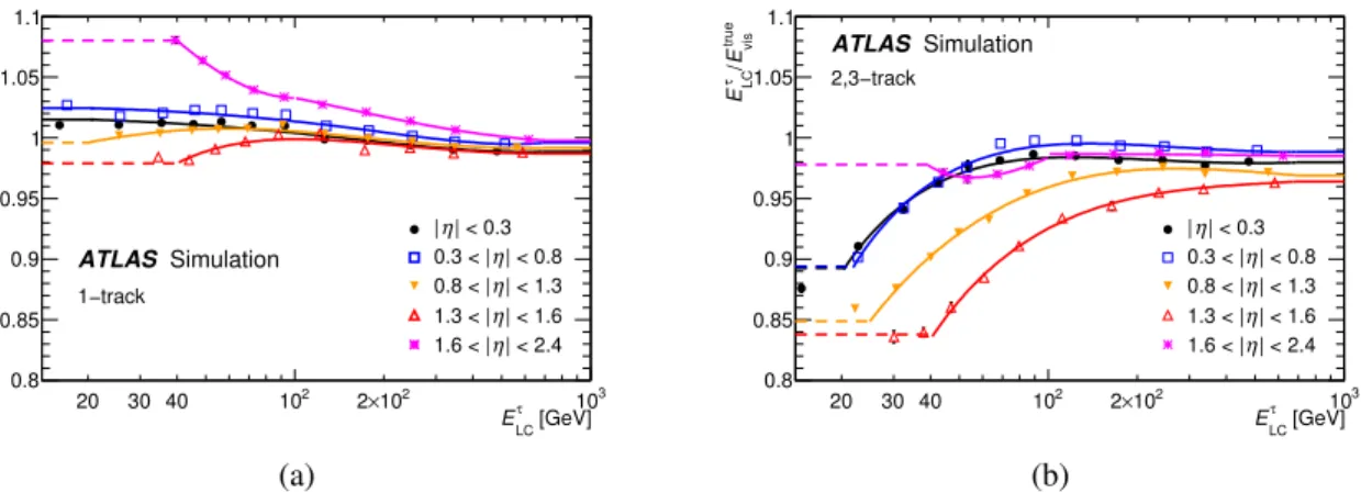
3.4 Hadronic Taus . . . 38

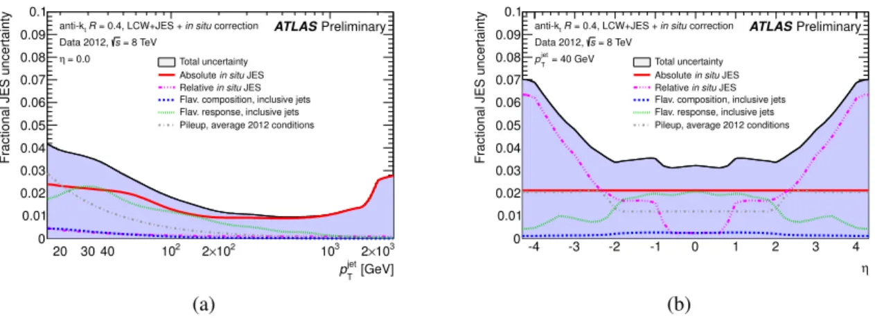
3.5 Jets . . . 45

3.6 Missing Transverse Energy . . . 47

4 Search for the Higgs Boson inH→τ τ Final State . . . 50

4.1 Signature ofH→τ τ Final State . . . 50

4.2 Background Processes . . . 51

4.3 Data and Simulation Samples . . . 54

4.3.1 Data Sample . . . 54

4.3.2 Simulation Samples . . . 54

4.4 Event Selection and Categorization . . . 57

4.4.1 Object Definition . . . 57

4.4.2 Event Selection and Categorization . . . 58

4.4.3 Signal and Control Regions . . . 62

4.5 Mass Reconstruction . . . 63

4.6 Background Model . . . 67

4.6.1 Z →τ τ Background . . . 68

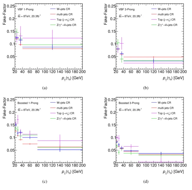
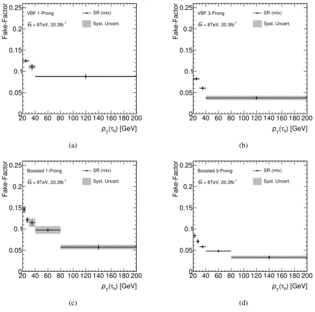
4.6.2 Fakeτ_had Background . . . 70

4.6.3 Top Background . . . 74

4.6.4 Z →ℓℓand di-boson Background . . . 76

4.6.5 Comparison between Observed Data and Background Modeling . . . 76

4.7 Multivariate Analysis . . . 81

4.7.1 Boosted Decision Tree (BDT) . . . 81

4.7.2 BDT Optimization . . . 83

4.7.3 Validation of BDT Output Distributions . . . 87

4.8 Systematic Uncertainties . . . 94

4.8.1 Theoretical Systematic Uncertainties . . . 94

4.8.2 Experimental Systematic Uncertainties . . . 95

4.8.3 Systematic Uncertainties on the Background Modeling . . . 97

4.9 Results of the Search for the Higgs Boson . . . 99

4.9.1 Signal Extraction Procedure . . . 99

4.9.2 Results of theH→τ_ℓτ_hadSearch . . . 100

4.9.3 Combination Results of theH →τ τ Search . . . 104

5 Study of CP Measurement in theτ τ Final State . . . 108

5.1 Overview of theH →τ_hadτ_hadAnalysis . . . 108

5.2 CP Observables in theH →τ τ analysis . . . 111

5.2.1 Transverse Spin Correlations . . . 112

5.2.2 Acoplanarity Angle . . . 112

5.2.3 CP Observables . . . 114

5.3 Event Selection and Observable Reconstruction . . . 121

5.3.1 Simulation of the CB-odd Higgs Boson Sample . . . 121

5.3.2 Event Selection and Categorization . . . 122

5.3.3 Observable Reconstruction . . . 125

5.4 Systematic Uncertainties . . . 130

5.5 Results of the CP Measurement . . . 131

5.5.1 Statistical Model . . . 131

5.5.2 Results . . . 131

6 Conclusions and Prospects . . . 133

A Additions for Chapter 4 . . . 135

A.1 Background Modeling . . . 135

A.2 Nuisance Parameters . . . 143

B Additions For Chapter 5 . . . 145

8

C ^HAPTER 1 Introduction

1.1 The Standard Model and the Higgs Boson

Current particle physics is described by the quantum field theory, so-called the Standard Model (SM).

The SM consists of six leptons and six quarks as elementary particles, and gauge fields are introduced to describe interactions between the particles. The gauge fields in the SM are required in order the symme- triesSU(3)_C ⊗SU(2)_L⊗U(1)_Y of the SM to be gauge symmetries, where interactions are mediated by mass-less bosons. TheSU(3)gauge symmetry describes the strong interaction between quarks and the gluon, while theSU(2)_L⊗U(1)_Y gauge symmetry [1] describes the electroweak interaction propa- gated by the photon and theW andZbosons, respectively. The Higgs mechanism [2–4] is introduced in order to provide particle masses without discarding the gauge-symmetry. The Higgs mechanism is based on the Higgs field that has a non-vanishing vacuum expectation value triggering spontaneous symmetry breaking. TheW andZboson masses are given by an interaction between the gauge field and the Higgs field, and the particle created by the Higgs field after the Higgs mechanism is called the Higgs boson.

The W andZ boson masses are predicted by this mechanism, and their expected values are consistent with measured values. The Higgs mechanism also provides lepton and quark (fermion) masses by intro- ducing a coupling between the Higgs boson and fermions, while their absolute values are determined by a measurement of the coupling constant, referred to as Yukawa coupling. In this section, an overview of the Higgs mechanism and the Yukawa coupling is given [5].

1.1.1 The Higgs Mechanism

The Higgs mechanism leads to the mass generation via spontaneous symmetry breaking. Spontaneous symmetry breaking is a process that a full symmetric system moves to a lower symmetry system, where the potential of the system settles into the energetically stable vacuum. In the Higgs mechanism, sponta- neous symmetry breaking is caused by a complex scalar doubletΦ, described as

Φ = (ϕ⁺

ϕ⁰ )

= 1

√2

(ϕ₀+iϕ₂ ϕ₃+iϕ₄

)

. (1.1)

The Lagrangian of the Higgs field is expressed by

L_Higgs = (D_µΦ)^†(D_µΦ)−V(Φ), V(Φ) = µ²(Φ^†Φ) +λ

4(Φ^†Φ)², (1.2)

whereDµis the covariant derivative andV(Φ)is the Higgs potential, which is parameterized by the the mass parameterµand self-coupling constantλ. The Lagrangian 1.2 is invariant under the transformation of SU(2)L⊗U(1)Y symmetry. While the coupling constant λis required to be λ > 0 for a stable vacuum, µ² can be considered in two scenarios. In case ofµ² > 0, the potentialV(Φ)is stable at the ground state of|Φ|= 0. On the other hand, in case ofµ² <0, the potential has a local maximum at

|Φ|²= −µ² 2λ = 1

2ν², (1.3)

whereν is the vacuum expectation value. If theΦtakes finite minimum value, theSU(2)_L⊗U(1)_Y symmetry is spontaneously broken. The ϕ⁺ and the imaginary part of ϕ⁰ are absorbed into massive W^± andZ bosons as their longitudinal modes. Such an absorption process is referred to as the Higgs mechanism. After the Higgs mechanism occurs, the complex scalar fieldΦcan be expressed by

Φ = 1

√2 ( 0

ν+h )

, (1.4)

where hrepresents the field that creates the Higgs boson. Using this equation, the Lagrangian can be expanded as

L_Higgs = 1

2(∂_µh)²+1

4g²W_µW^µ(ν+h)² + 1

8(ν√

g²+g^′2)(ν+h)²Z_µZ^µ + µ²

2 (ν+h)²− λ

16(ν+h)⁴, (1.5)

where theW andZ represents the physicalW andZfields, andgandg^′representsSU(2)_LandU(1)_Y gauge coupling constants, respectively. The Higgs mechanism generates mass terms ofW,Z and the Higgs bosons leaving the photon and gluon mass-less in the SM Lagrangian including 1.5. The masses of theW andZbosons are extracted from equation (1.5) as:

m_H =√

2λν², m_W = gν

2 , m_Z = ν 2

√g²+g^′2. (1.6)

The W andZ boson masses (m_W andm_Z) can be predicted by the SM as shown in equation (1.6), those are consistent with the experimental results. However, the Higgs boson mass (m_H) contains a free parameterλ, that is the Higgs self-coupling constant.

1.1.2 Yukawa Couplings

The Higgs field in the SM also generates fermion masses by introducing interactions between the same complex scalarSU(2)doubletΦ, a left-handed fermion SU(2) doubletΨ_Land a right-handed fermion singletΨ_R, referred to as Yukawa couplings. The general Lagrangian for such interactions can be de-

10

scribed as

L_{Y ukawa} =−Y_f( ¯Ψ_LΨ_R)Φ +h.c., (1.7)

whereY_f is the Yukawa coupling constant between the Higgs boson and fermions, andh.c.represents the Hermitian conjugate. By introducing the spontaneous symmetry breaking with the Higgs field of equation (1.4), the Lagrangian is expanded as

L_{Y ukawa}=−νY_f

√2( ¯Ψ_LΨ_R+ ¯Ψ_RΨ_L)(1 +h

ν). (1.8)

Thus, the fermion mass is provided as

m_f = νY_f

√2. (1.9)

In case of quarks, the field provides a mass term also for up side of theSU(2)quark doublet by converting the Higgs doubletΦtoΦ^′. The general Lagrangian for quark Yukawa couplings is described as:

L_{Y ukawa} = −Y_d( ¯Ψ_d,LΨ_d,R)Φ−Yu( ¯Ψu,LΨu,R)Φ^′+h.c.

= −νY_d

√2( ¯Ψ_d,LΨ_d,R+ ¯Ψ_d,RΨ_d,L)(1 + h

ν)−νY_u

√2( ¯Ψ_u,LΨ_u,R+ ¯Ψ_u,RΨ_u,L)(1 +h ν), Φ^′ =

(−ϕ₀ ϕ⁻

)

= 1

√2

(ν+h 0

)

, (1.10)

.

In both cases, the fermion mass can be described by the equation (1.9). While the Higgs mechanism is an excellent theory that explains generation mechanism of both boson and fermion masses, it has an uncertain aspect that cannot predict absolute values of masses since the Yukawa coupling constantsY_f are free parameters. These values must be experimentally measured for the verification of the Higgs mechanism, which is one of main scopes of this thesis.

1.2 Phenomenology of the Higgs Boson at the LHC

1.2.1 Production Processes

The Higgs boson production at the LHC is dominated by four processes: gluon fusion (ggF), vector boson fusion (VBF), vector boson associated (V H) and top quark associated (t¯tH) processes. Leading- order (LO) level Feynman diagrams of signal production processes considered in this analysis are shown in Fig. 1.1.

The ggF process has the largest cross section in the four processes. The Higgs boson produced via a heavy quark loop from gluons, where a heavy quark is dominated by a top quark loop due to a large Yukawa coupling. Thus, the discovery of the ggF indicates an indirect confirmation of Yukawa coupling.

g

g f

f

f H

(a) Gluon fusion (ggF)

q (’)

q q

q(’)

±/Z W

/Z

±

W

H

(b) Vector boson fusion (VBF)

q’

q

±/Z W

±/Z W

H (c) Vector boson associated (V H)

g g

t

t t t

H

(d) top pair associated (t¯tH)

Fig. 1.1: Leading-order Feynman diagrams of the Higgs boson production processes at the LHC.

The final state of the process is only the Higgs boson, and therefore the process is relatively hard to separate from background events in the analysis. The VBF process has the second largest cross section.

In this process, typically two jets in the forward and backward regions of the detector are associated.

The characteristic signature is useful to suppress background events in the analysis. The VBF process provides the information of the direct coupling of the Higgs boson and weak gauge bosons. In theV H process, the Higgs boson is produced associated with the vector boson (Z orW boson). In this process, there are several final states depending on decay products of the vector boson. Especially, the final state contains leptons is effective to suppress background, such as multi-jet events. Thet¯tHprocess has the Higgs boson is produces associated with top quark pair. This process provides the information of the top Yukawa coupling. However, this process does not contribute significantly to signal regions in this thesis due to the smallest cross section. The production cross section for each process and inclusive cross sections at√

s= 7,8and14TeV are shown in Fig. 1.2.

1.2.2 Decay Modes and Experimental Search Channels

The branching ratio of the Higgs boson depends on masses of the decay products as shown in Fig. 1.3 (a) because the Higgs boson coupling is proportional to the masses. In the interested region around the measured Higgs boson mass ofm_H ∼125GeV, the dominant decay mode is theH →b¯bdecay with the branching ratio of∼57.7%. The second largest decay mode is theH→W W decay with the branching ratio of∼21.5%. This decay mode is suppressed in the region since one ofW bosons can be produced with on-shell. The third largest decay mode is theH →τ τ decay with the branching ratio of∼6.3%.

Although the Higgs boson decays into several particles, certain combinations of production processes and decay modes can be used taken into account trigger limitations and background contributions. The

12

[GeV]

MH

100 150 200 250 300

H+X) [pb] →(pp σ

10-2

10-1

1 10 102

= 8 TeV s

LHC HIGGS XS WG 2012

H (NNLO+NNLL QCD + NLO EW) pp →

qqH (NNLO QCD + NLO EW)

→ pp

WH (NNLO QCD + NLO EW) pp →

ZH (NNLO QCD +NLO EW) pp →

ttH (NLO QCD) pp →

(a)

[GeV]

MH

100 150 200 250 300

H+X) [pb] →(pp σ

1 10 102

LHC HIGGS XS WG 2012

=14 TeV s H+X at pp →

=8 TeV s H+X at pp →

=7 TeV s H+X at pp →

(b)

Fig. 1.2: (a) Production cross sections of the SM Higgs boson of main production processes at √ s = 8TeV and (b) inclusive cross sections at√

s= 7,8and14TeV as a function ofm_H.

product of production cross section times branching ratio (event rate) for each important experimental search channel at the LHC is shown in Fig. 1.3 (b). The H → τ τ channel has the largest event rate around the region ofmH ∼125GeV.

[GeV]

MH

80 100 120 140 160 180 200

Higgs BR + Total Uncert

10-4

10-3

10-2

10-1

1

LHC HIGGS XS WG 2013

b b τ

τ

µ µ c c

gg

γ

γ Zγ

WW

ZZ

(a)

[GeV]

MH

100 150 200 250

BR [pb]×σ

10-4

10-3

10-2

10-1

1 10

LHC HIGGS XS WG 2012

= 8TeV s

µ l = e,

ντ µ, ν

e, ν ν = q = udscb

b νb l±

→ WH

b

-b

+l

→ l ZH

b

→ ttb ttH τ-

τ+

→ VBF H

τ-

τ+

γ γ

q νq l±

→ WW

-ν νl l+

→ WW

q

-q

+l

→ l ZZ

ν

-ν

+l

→ l ZZ

l-

l+

l-

l+

→ ZZ

(b)

Fig. 1.3: (a) Branching ratios of the SM Higgs boson and (b) production cross sections at√

s= 8TeV times branching ratio for experimentally important processes (b) as a function ofmH.

1.2.3 Experimental Status of the Higgs Boson Searches

The Higgs boson has been searched experimentally for a long time since the Higgs mechanism was proposed. While the Higgs boson mass is a free parameter in the SM as mentioned in Section 1.1.1, the mass range can be constrained by mass measurements of W boson and top quark because the W boson mass depends on the top quark and the Higgs boson masses through radiative effects [6]. the Higgs boson is predicted to contribute their measured masses through loop corrections. The first Higgs boson search was indirectly performed based on two dimensional mass fit ofW boson and top quark by the LEP experiments [7], where the top quark mass was estimated by electroweak measurements. This indirect search was updated with the precisely measuredW boson mass from the LEP2 and the Tevatron, and the directly measured top quark mass from the Tevatron [8]. The Higgs boson mass is favoured in a lower mass range (30GeV< m_H <300GeV) by the indirect search.

Based on the result, the direct Higgs boson searches were performed at the LEP/LEP2 and the Tevatron experiments. The LEP2 experiments finally set a lower exclusion limit of the Higgs boson mass of m_H > 114GeV at95% confidence level using the vector boson associated production (V H), where a main contribution from the (H → b¯b)(Z → qq) final state [9]. The Tevatron experiments (CDF¯ and DØexperiments) are also performed the direct search with several experimental search channels.

These channels are combined, and the Tevatron set an exclusion limit of the Higgs boson mass of two regions: 90GeV < m_H < 109GeV and 149GeV < m_H < 182GeV at 95%confidence level [10].

Main contributions of lower and higher limits are from theV H →b¯band theH →W W^∗ →ℓ⁺νℓ⁻ν¯ channels, respectively. TheH → τ τ search was performed in the CDF experiment, the upper limit of the SM cross section times branching ratio(σ_SM×B(H →τ τ))is 16.4 atm_H = 125GeV [11].

The LHC started the operation in 2010, and the ATLAS and CMS experiments collected data with the center-of-mass energy of7TeV in 2010-2011 and8TeV in 2012. In July 2012, both experiments reported the discovery of a new particle, that is most likely the Higgs boson, with a mass of about125GeV, the integrated luminosities are 4.8(5.1)fb⁻¹1 at√s = 7TeV and5.8(5.3)fb⁻¹ at √s = 8TeV for the ATLAS (CMS) experiment [12, 13]. The discovery was mainly provided from diboson decay channels, i.e., theH→γγ,H→ZZ andH→W W channels. Figure 1.4 shows thep-value of the background- only hypothesis as a function ofmH, which is obtained from the combination of results from theH →γγ andH →ZZ andH →W W searches. With full dataset in 2011-2012, corresponding to an integrated luminosity of up to 25 fb⁻¹, the measurement of spin and parity quantum numbers of the discovered Higgs boson was performed by both experiments. The results are consistent with the SM prediction of the Higgs boson withJ^P = 0⁺[14] (see Section 1.3.2).

The discovery of the Higgs boson was made by the H → γγ, H → ZZ and H → W W channels.

Therefore, it is important to measure properties of the discovered Higgs boson for understanding the na- ture of electroweak symmetry breaking. The current main topics of the Higgs analysis are an observation of the coupling between the Higgs boson and ferimons, and its property measurements.

14

[GeV]

mH

110 115 120 125 130 135 140 145 150

0Local p

10-11

10-10

10-9

10-8

10-7

10-6

10-5

10-4

10-3

10-2

10-1

1

Obs.

Exp.

σ

±1 Ldt = 5.8-5.9 fb-1

∫

= 8 TeV:

s

Ldt = 4.6-4.8 fb-1

∫

= 7 TeV:

s

ATLAS

σ 0

σ 1

σ 2

σ 3

σ 4

σ 5

σ 6

Fig. 1.4: Observed localp₀(solid line) as a function ofm_H. The dashed curve shows the expected local p0under the hypothesis of the SM Higgs boson signal at that mass with its plus/minus one sigma band.

The horizontal dashed lines indicate thep-values corresponding to significances of 1 to 6σ[12].

1.2.4 Phenomenology of theH →τ τ

TheH →τ τ channel plays an important role in the Higgs boson search as fermion channels due to its high event rate and relatively clean signature in the final state. This section introduces properties and decay modes of aτ lepton, and an experimental signature of theH →τ τ final state.

Tau Lepton Decays

τ

W

ν

l

ν

τ

W

ν

q q’

(b)

Fig. 1.5: Feynman diagrams ofτ lepton decay for (a) leptonically and (b) hadronically.

The tau lepton [15] is the heaviest lepton with a mass of1.78GeV, a mean life time of(290.6±1.0)× 10⁻¹⁵s and an average decay length of87.11µm. The tau lepton typically decays before reaching the active region of the ATLAS detector. The decay is classified into leptonicallyτ →ℓν_ℓν_τ (ℓ=e/µ)and hadronicallyτ →hadronsντ, as shown in Fig. 1.5. The leptonic decay is further classified into electron

and muon decays, and the total branching ratio is∼35%. The lepton from the leptonic decay is referred to asτ_ℓin this thesis. The hadronic decay has several decay modes corresponding to the number and kind of hadrons, and the total branching ratio is∼65%. Decay products of the hadrinic decay are referred to asτhad in this thesis. One and three charged hadrons from the hadronic decay are referred to as 1-prong and 3-prong decay, respectively. The hadronic decay is further classified corresponding to the number of neutral hadrons, mainly neutral pions. A typical process of the decay into 1-prong τhad associated with one neutral pion is τ^± → ρ^±(

→π^±π⁰)

ν_τ process, and associated with two neutral pions is τ^± → a^±₁ (

→π^∓π⁰π⁰)

ν_τ process, whereρanda₁are short-lived mesons with a mass of∼770MeV and∼ 1260MeV, respectively. A typical process of the 3-prong decay isτ^± → a^±₁ (→π^±π^∓π^±)ν_τ process. Dominant decay modes of a tau lepton are listed in Table 1.1 with their branching ratios.

Decay modes Branching ratio [%]

leptonic decay 35.24±0.08 τ⁻→e⁻ν_eν_τ 17.83±0.04 τ⁻→µ⁻νµντ 17.41±0.04 hadronic decay 64.76±0.21 τ⁻→π⁻ν_τ 10.83±0.06 τ⁻→π⁻π⁰ν_τ 25.52±0.09 τ⁻→π⁻π⁰π⁰ν_τ 9.30±0.11 τ⁻→π⁻π⁰π⁰π⁰ν_τ 1.05±0.07 τ⁻→K⁻ν_τ 0.700±0.010 τ⁻→K⁻π⁰ν_τ 0.429±0.015 τ⁻→π⁻π⁻π⁺ν_τ 8.99±0.06 τ⁻→π⁻π⁻π⁺π⁰ν_τ 2.70±0.08

Table 1.1: Summary of tau lepton decay modes and corresponding branching ratios [15].

H →τ τ channel

Corresponding to the tau lepton decay, theH → τ τ channel can be classified into three channels: the fully leptonic channel H → τ_ℓτ_ℓ, the fully hadronic channel H → τ_hadτ_had, and the lepton-hadron channel H → τ_ℓτ_had, with branching ratios of12.4%, 42% and 45.6%, respectively. Experimental search sensitivity of each channel is determined corresponding to the branching ratio and the number of neutrinos fromτ lepton decays (see Section 4.1). The lepton-hadron channel has the largest event rate and a clean final state due to the presence of the lepton, and they leads this channel to have the highest sensitivity in theH→τ τ search. While the fully hadronic channel has the same degree of the branching

16

ratio with the lepton-hadron channel, this channel suffers from large multi-jet backgrounds. This channel is the second channel in theH →τ τsearch. As a feature of this channel, this channel is able to precisely reconstruct kinematic distributions than other two channels due to a less number of neutrinos in the final state, and it is useful in both the search and property measurements of the Higgs boson. While the fully leptonic channel has the cleanest final state because of two leptons, its branching ratio is the smallest and the resolution of reconstructed kinematic distributions is lower than other channels due to the presence of four neutrinos in the final state. This channel is the third channel in theH → τ τ search. The three channels are independently analyzed, and then theH →τ τ search result are obtained by a combination of three channels.

1.3 CP Measurement of the Higgs Boson

1.3.1 Two Higgs Doublet Model

After the observation of the coupling between the Higgs boson andτ leptons, one of the most important remaining question is whether the observed Higgs boson is the SM Higgs boson or a part of an extended Higgs sector predicted by BSM theory models. The SM predicts the Higgs boson has a CP-even state, while a CP-odd Higgs boson appears in several BSM theories based on the two Higgs doublet model (2HDM) [16, 17], which is a minimal extension from the SM Higgs sector. In the 2HDM, two complex scalar doubletsΦ1andΦ2are introduced as:

Φ_i =

( ϕ⁺

√1

2(ν_i+h_i+iz_i) )

, (i= 1,2). (1.11)

Introducing the two doublets, the general potential of the Higgs fieldV(Φ₁,Φ₂)can be expressed by:

V(Φ₁,Φ₂) = m²₁₁Φ^†₁Φ₁+m₂₂² Φ^†₂Φ₂−(m₁₂Φ^†₁Φ₂+h.c) + λ₁

2 (Φ^†₁Φ₁)²+λ₂

2 (Φ^†₂Φ₂)² + λ3(Φ^†₁Φ1)(Φ^†₂Φ2) +λ4(Φ^†₁Φ2)(Φ^†₂Φ1) +λ₅

2

[(Φ^†₁Φ2)²+h.c.]

, (1.12)

whereλ1−5 represents coupling constants, andm11,m22andm12are mass parameters. The Higgs dou- blets 1.11 have eight degrees of freedom in total. After spontaneous symmetry breaking, three of them are absorbed to give mass to theW andZbosons. Assuming a CP-symmetry conservation, the remaining five degrees of freedom correspond to five physical Higgs bosons: two neutral CP-even bosons (hand H), one neutral CP-odd boson (A) and a pair of charged bosons (H^±). After all, the parameters in the above Higgs potential are converted into the masses of five bosons, the ratio of the vacuum expectation values of two doublets (tanβ ≡ν₂/ν₁), the mixing angle between two CP-even bosons (α) and the po- tential parameter (m²₁₂). In addition, this model can be classified into two types, referred to as type I and type II 2HDM, those are distinguished by the structure of Yukawa coupling. All fermions couple to only Φ₂ in type I 2HDM, while up-type fermions couple toΦ₂and down-type fermions couple toΦ₁in type II. Although the choice of two types depends on theory models, the CP-even and CP-odd Higgs bosons

are included in both types. The typical examples of the theory including two Higgs doublets are follow- ings: the minimal super-symmetric SM (MSSM) [18–21], the axion model [22] and the baryogenesis model [23]. The measurement of the CP state of the discovered Higgs boson is of primary importance to determine whether it is the SM (CP-even) Higgs boson or the BSM (CP-odd) Higgs boson.

1.3.2 Experimental Status of the CP Measurements of the Higgs Boson

With the discovery of the Higgs boson, the measurement of the spin and CP quantum numbers were performed by the ATLAS and the CMS experiments based on di-boson decay channels: theH → γγ, theH→ZZ^∗ →4ℓand theH→W W^∗ →ℓνℓνchannels [14,24]. The analysis dataset corresponding to an integrated luminosity of 4.6(5.1)fb⁻¹ collected at√s = 7TeV and20.3(19.7)fb⁻¹ collected at

√s= 8TeV. In order to test the SM prediction of the Higgs boson withJ^P = 0⁺, alternative hypotheses ofJ^P = 0⁻,1⁺,1⁻ and2⁺are studied. Focusing on theH → ZZ^∗ → 4ℓas a typical example, the measurement was performed with total eight discriminant variables, five angle variables in the four- body decay, and invariant masses of lepton pairs and four leptons. Multivariate analysis was used to discriminate the J^P = 0⁺ hypothesis from each alternative hypothesis. The results exclude all of the alternative models in favour of the SM Higgs boson hypothesis at more than 97.8%confidence level.

Figure 1.6 shows an example distribution of the test statistics of the Higgs boson withJ^P = 0⁺(SM), and with J^P = 0⁻ (BSM) hypotheses in the ATLAS experiment, where the exclusion limit is 97.8%

confidence level. Although the result indicates that the Higgs boson in di-boson channels is consistent with the SM, it is important to test the consistency with the fermion final states. Moreover, the CP-odd Higgs boson must decay into di-boson via a fermion loop, so that the direct CP measurement can be performed by only fermion final states. This is the primary motivation of the CP measurement in theτ τ final state.

18

q~

-30 -20 -10 0 10 20 30

Arbitrary normalisation

10-5

10-4

10-3

10-2

10-1

1

10 ATLAS H → ZZ* → 4l

= 7 TeV, 4.5 fb-1 s

= 8 TeV, 20.3 fb-1 s

νµν

→e WW*

→ H

= 8 TeV, 20.3 fb-1 s

Data

+ SM 0 0−

Fig. 1.6: An example distribution of the test statisticq for the combination of theH →ZZ^∗ → 4ℓand theH → W W^∗ →ℓνℓν channels in the ATLAS experiment. The solid black line represents observed data, while the solid blue line and the dashed red line represent the Higgs boson withJ^P = 0⁺ (SM), and withJ^P = 0⁻(BSM) hypotheses, respectively [14].

C ^HAPTER 2

LHC and ATLAS detector

The analysis in this thesis uses the data collected by the ATLAS (A Toroidal Lhc ApparatuS) detector in collisions of proton-proton delivered by the Large Hadron Collider (LHC). In this chapter, the LHC accelerator complex and the ATLAS detector configurations are summarized.

2.1 Large Hadron Collider

The LHC [25] is proton-proton circular collider located at European Organization for Nuclear Research (CERN) in Geneva, Switzerland. The collider is arranged in an underground circular tunnel at a depth of ranging from 50m to 175m with a circumference of 27km, which was initially constructed for the Large Electron Positron Collider (LEP) experiment. The LHC is designed to provide center of mass energies up to√

s= 14TeV with instantaneous luminosity of over 10³⁴cm⁻²s⁻¹. The accelerator chain located at CERN increases the energy of proton beams in stages and the chain is enable to be achieved such performance finally at the LHC main ring.

2.1.1 Accelerator Chain

The protons, obtained from ionizing hydrogen gas, are injected to a linear accelerator (LINAC2) at first, and they are accelerated to50MeV. The protons are then grouped into bunches by Radio-Frequency (RF) cavities, and the proton bunches are injected into a series of accelerators : Proton Synchrotron Booster (PSB), Proton Synchrotron (PS), Super Proton Synchrotron (SPS). The proton beam is accelerated and the energy is increased to 1.4GeV, 25GeV and 450GeV, respectively. Finally, the proton beam is injected into the LHC main ring and they are accelerated to the designed energy. The proton accelerator chain is summarized in Fig. 2.1.

2.1.2 LHC Run-1 Data Taking

The first run of the LHC, referred to as “LHC Run-1”, was successfully finished in 2013. The initial design of the LHC is to collide proton beams at √s = 14TeV with instantaneous luminosity of over 10³⁴ cm⁻² s⁻¹. During initial operation in 2008, a large section of the superconducting magnets in the LHC are quenched. It was decided to reduce the energy of the LHC for the initial run during a repair of these magnets and an addition of quench protections. After the repairing, in 2010 and 2011, the LHC was operated with the energy of proton beams of 3.5TeV, producing center-of-mass energy

20

to as “Run”. The Run is subdivided into “luminosity block”, which holds each integrated luminosity information. The ATLAS monitoring systems of each sub-detector and dedicated data quality shifters check qualities of the recorded data for each luminosity block. The quality information of luminosity block is listed run by run, so-called “Good Run List”, and it is used in physics analyses to ensure that the analyzed data is not affected by detector failures. The integrated luminosity of the good quality data in 2011 and 2012 is4.25fb⁻¹ and20.3fb⁻¹, respectively. Figure 2.2 (a) shows the integrated luminosity with respect to operation times for delivered, recorded and good quality data.

Pileups

Due to a high instantaneous luminosity, single bunch crossing produces multiple proton-proton inter- actions, so-called “pileup”. The number of interactions per bunch crossing depends on run conditions, while typical events have the average number of 20.7 (9.1) in 2012 (2011) data. Figure 2.2 (b) shows distributions of the mean number interactions per crossing< µ >in 2011 and 2012. The pile-up events affects adversely to physics analyses because additional tracks and energy deposits of particles from the pileup events give ambiguity of physics object reconstructions and identifications. In order to model pileup events in simulation samples, a dedicated< µ >rescaling is performed (see Section 4.3.2).

Month in Year Jan Apr Jul Oct Jan Apr Jul Oct

-1fbTotal Integrated Luminosity

0 5 10 15 20 25 30

ATLAS Preliminary

= 7 TeV s 2011,

= 8 TeV s 2012, LHC Delivered

ATLAS Recorded Good for Physics

fb-1 Delivered: 5.46

fb-1 Recorded: 5.08

fb-1 Physics: 4.57

fb-1 Delivered: 22.8

fb-1 Recorded: 21.3

fb-1 Physics: 20.3

(a)

Mean Number of Interactions per Crossing

0 5 10 15 20 25 30 35 40 45

/0.1]-1Recorded Luminosity [pb

0 20 40 60 80 100 120 140 160

180 ATLASOnline Luminosity

> = 20.7 , <µ Ldt = 21.7 fb-1

∫

= 8 TeV, s

> = 9.1 , <µ Ldt = 5.2 fb-1

∫

= 7 TeV, s

(b)

Fig. 2.2: (a) The integrated luminosity with respect to operation time for delivered (green), recorded (yellow) and good quality data (blue). (b) The< µ >distributions in 2011 (blue) and 2012 (green) [27].

2.2 ATLAS Detector

The ATLAS [28–30] detector is a general purpose detector located at one of the proton-proton collision point of the LHC, and it is designed to verify the wide range of the interests of the SM (e.g. Higgs boson, top quark and so on) and search for the BSM physics at the LHC energy scale. To study these physics interests, the ATLAS detector reconstructs and identifies a wide range of objects, i.e. electrons, photons, muons,τ_hads, jets and the missing transverse energy (E^miss_T ).

22

The ATLAS detector consists of a barrel region and two endcap region with several sub-detector systems, Tracking Detectors, Magnetic Systems, EM (Electromagnetic) Calorimeter, Hadron Calorimeter and Muon Spectrometer, in order from inner to outer. Schematic view of the ATLAS detector is shown in Fig. 2.3.

Fig. 2.3: Schematic view of the ATLAS Detector Systems. The dimensions are 25 m in height and 44 m in length. The overall weight of the detector is approximately 7 kilotons [28].

In the ATLAS coordinate system, the z axis is defined as the beam direction, and the x and y axis are defined as horizontal and vertical axes towards the center of the LHC ring, respectively. The azimuthal angle ϕis defined with respect to the x axis between−π andπ, whereϕ= 0represents the positive x axis. The polar angleθis defined with respect to the z axis between 0 andπ, whereθ= 0represents the positive z axis. The pseudo rapidity η = 1/2 ln tan(θ/2)is often used instead of the polar angle. The distance between objects inη−ϕplane is defined as∆R=√

∆η²+ ∆ϕ². The transverse momentum and energy are defined asp_T=p×sinθandE_T=Esinθin the x-y plane, respectively.

2.2.1 Inner Detector

The tracking system [31, 32], referred to as the Inner Detector (ID), is located at innermost part of the ATLAS detector in order to measure the momentum of charged particles and to determine the location of vertices. The ID consists of three sub-detectors, silicon pixel tracker (Pixel) [33, 34] ,semiconducting silicon micro-strip tracker (SCT) [35–37] and transition radiation tracker (TRT) [38–40]. The solenoid magnet system surrounds of the ID, which generates a 2 Tesla magnetic field. The layout and the cover- age of the ID are summarized in Fig. 2.4 and Figure 2.5, respectively.

Fig. 2.4: Cut-away view of the ATLAS tracking detectors [28].

Envelopes Pixel SCT barrel SCT end-cap

TRT barrel TRT end-cap

255<R<549mm

|Z|<805mm 251<R<610mm 810<|Z|<2797mm

554<R<1082mm

|Z|<780mm 617<R<1106mm 827<|Z|<2744mm

45.5<R<242mm

|Z|<3092mm Cryostat PPF1

Cryostat Solenoid coil

z(mm)

Beam-pipe Pixel

support tube

SCT (end-cap) TRT(end-cap)

1 23 4 567 8 9 10 11 12 1 2 3 4 5 6 7 8

Pixel 400.5

495 580

650 749

853.8 934

1091.5 1299.9

1399.7

1771.4 2115.2 2505 2720.2

00 R50.5 R88.5 R122.5 R299 R371 R443 R514 R563 R1066 R1150

R229 R560 R438.8 R408 R337.6 R275

R644 R1004 2710 848

712 PPB1

Radius(mm)

TRT(barrel)

SCT(barrel)

Pixel PP1 ID end-plate 3512

Pixel

400.5 495 580 650 0

0 R50.5 R88.5 R122.5

R88.8 R149.6

R34.3

Fig. 2.5: Plan view of a quarter-section of the ATLAS tracking detectors with active dimensions and envelopes [28].

Pixel Detector

The Pixel detector is the innermost detector consisting of semiconduction silicon sensors with the pixel size50×400µm², with a coverage up to|η|= 2.5. The space point measurements of charged particle are performed with high resolution due to such small pixel size of the sensors. The innermost layer of this detector is located at the radius of51mm from the LHC beam pipe. The typical resolutions are (σ_ϕ, σ_z) = (10µm,115µm)in the barrel region, and(σ_ϕ, σ_r) = (10µm,580µm)in the endcap region.

24

The total number of readout channels is∼80.4million.

Semi-Conductor Tracker (SCT)

The SCT is the second innermost detector consisting of eight strip layers, with a coverage up to|η|= 2.5, The unit of the SCT module consists of two layers of semiconducting silicon strip sensors with a pitch of80µm. The two layers are mounted in each module with a small stereo angle of40mrad to measure the coordinates of ϕand z. The typical resolutions of each module is(σ_ϕ, σz) = (17µm,580µm) in the barrel region, and(σ_ϕ, σ_r) = (17µm,580µm)in the endcap region. In total, the number of readout channels is∼6.3million.

Transition Radiation Tracker (TRT)

The TRT is the outermost detector with a coverage up to|η| < 2.0. The TRT consists of straw tubes filled with a xenon based mixture gas with a gold plated tungsten wire. The length of each tube is 144cm and37cm in the barrel and endcap region, respectively. Average 30 hits (maximum 36 hits) per track are provided by the TRT, and it allows to perform precision tracking. The TRT uses the transition radiation, which is emitted by charged particles when it passes a boundary of two dielectric materials.

The intensity of the transition radiation is proportional to the Lorentz factor γ of the particle, which enables to the particle identification and the separation between electron and charged pion.

2.2.2 Calorimeters

The calorimeter system is located on the outside of the ID to measure the particle energy, with a coverage up to |η| < 4.9. The system consists of the electromagnetic (EM) and hadron calorimeters. The EM calorimeters are designed to be sensitive to the electromagnetic interactions in order to measure the energy of electrons and photons, while the hadron calorimeters are sensitive to hadronic interaction to measure the hadron energy. A cut-away view of the calorimeter system is shown in Fig. 2.6.

Electromagnetic Calorimeter

The EM calorimeter consists of∼ 1.5mm accordion-shaped lead plates as absorbers and2.1mm gaps filled with the liquid argon as active layers. The energy of charged particles are measured by detecting ionization of charged particles inside the liquid argon. The maximum drift time is 450ns by applying a high voltage of∼2,000V. This calorimeter separately consists of one cylindrical barrel calorimeter (|η|<1.475) with a small gap of4mm at|z|= 0and two wheel endcap calorimeters (1.375<|η|<

3.2). Each calorimeter contains three different layers for high angular resolution and to detect full shower shapes. The first layer is mounted with a granularity of∆η×∆ϕ= 0.0031×0.098and4.3X₀radiation length, referred to as strip layer. It allows to identifyπ⁰ →γγdecays, which is one of main background to photons [41] and is used in the identification of hadronically decayingτ lepton (see Section 3.4). The

Fig. 2.6: Cut-away view of the ATLAS calorimeter system [28].

second layer has a granularity of ∆η×∆ϕ = 0.025×0.0245with 16 X0 radiation length, and the most of energy from EM shower is measured by this layer. The third layer measures the tails of EM shower, and it enables to distinguish EM showers from hadronic showers. The granularity of this layer is

∆η×∆ϕ= 0.050×0.025. In addition to three layers, one11mm thin layer, referred to as pre-sampler, is mounted in front of the strip layer, with a granularity of∆η×∆ϕ= 0.025×0.1. The pre-sampler covers the range of |η| < 1.8to correct the energy loss in materials before the EM calorimeter. A schematic view of the barrel module of the EM calorimeter is shown in Fig. 2.7.

Hadron Calorimeter

The hadron calorimeter is mounted surrounding the EM calorimeter, and it consists of one barrel calo- rimeter (|η|<1.7), two endcap hadron calorimeters (1.5<|η|<3.2). The barrel calorimeter uses steel plates as absorber and scintillation tiles as active material, with a granularity of∆η×∆ϕ= 0.1×0.1. The scintillation photons are guided by wavelength shifter fibers, and they are read out by photo-multiplier tubes. The endcap calorimeters use coppers and liquid argon gas as absorber and active media, respec- tively. Each calorimeter has the total thickness of 10 interaction lengths, it is sufficient to decrease punch-trough hadrons.

Additionally, the forward calorimeter is mounted to cover higher pseudo-rapidity region of3.1<|η|<

4.9. This calorimeter is combined with EM and hadron calorimeters. The EM calorimeter uses copper, which length is optimized for EM interaction, as absorber, while the hadron calorimeter uses tungsten as absorber. Both calorimeters are filled with liquid argon gas as active media.

26

∆ϕ = 0.0245

∆η = 0.025 37.5mm/8 = 4.69 mm

∆η = 0.0031

∆ϕ=0.0245 36.8mmx4

=147.3mmx4

Trigger Tower

Trigger Tower

∆ϕ = 0.0982

∆η = 0.1

16X₀

4.3X0

2X0

1500 mm

470 mm

η ϕ

η = 0

Strip cells in Layer 1

Square cells in Layer 2 1.7X₀

Cells in Layer 3

∆ϕ×∆η = 0.0245×0.05

Fig. 2.7: Schematic view of the barrel module of the EM calorimeter [28].

2.2.3 Muon Spectrometer

The outermost detector in the ATLAS detector is the Muon Spectrometer (MS) with a coverage up to

|η| = 2.7. The cut-away view of the MS is shown in Fig. 2.8. The MS consists of two precision tracking chambers and two trigger chambers, with air-core toroid magnet system. The muon momentum is measured from the deflection of the muon trajectory in the magnetic field. The two precision chambers consist of three layers of the Monitored Drift Tubes (MDT) for the pseudo-rapidity range of|η| < 2.0 and two layers of the Cathode Strip Chambers (CSC) for 2.2 < |η| < 2.7. The MDT are made from multi-layers of tubes, while the CSC is multi-wire proportional chambers. Both chambers are filled with Ar/CO2mixture gas. Since the MDT and the CSC chambers require a wide time window of∼700µs, two dedicated trigger chambers are equipped to provide fast responses, which satisfies the ATLAS level 1 trigger requirement of selecting events in every25ns. The Resistive Plate Chambers (RPC) consists of three layers for the barrel region (|η|<1.05) and the Thin Gap Chambers (TGC) consists of three layers for the endcap region (1.05<|η|<2.4).

2.2.4 Trigger and Data Acquisition System

An average bunch crossing rate during data taking in 2011 and 2012 is ∼ 20MHz, and it does not allow to continuously read out all information from the ATLAS detector due to limitations of the ATLAS

Fig. 2.8: Cut-away view of the ATLAS muon spectrometer [28].

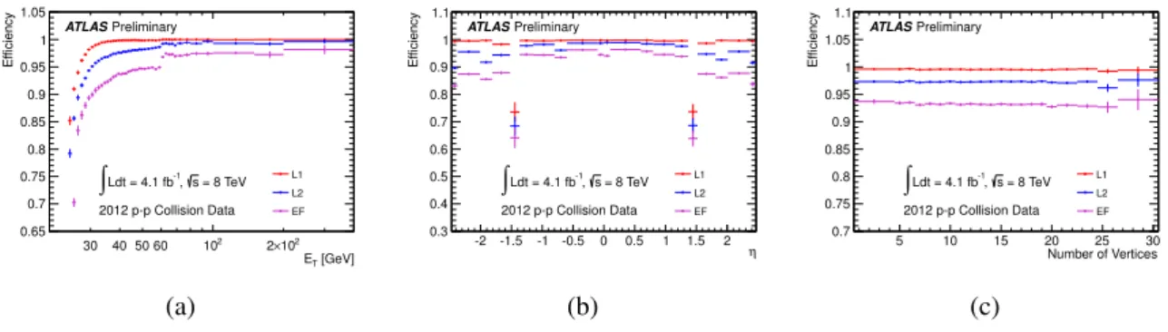
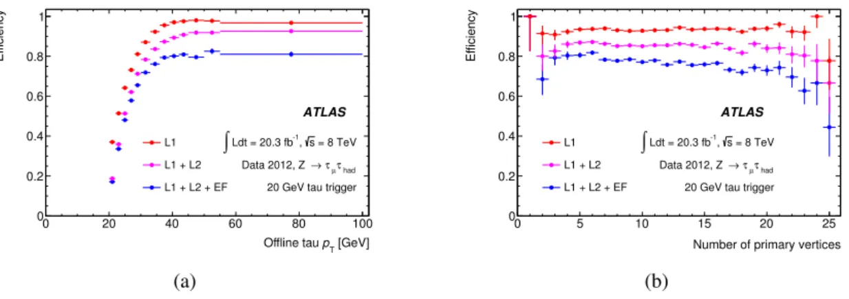
storage and computing systems. Therefore, a trigger system is necessary to efficiently select interesting events. The ATLAS trigger system consists of three levels: the hard-ware based level 1 (L1) trigger, and the soft-ware based Level 2 (L2) and Event Filter (EF) triggers.

The L1 trigger makes trigger decisions within an average processing time of 2.5µs using the limited information form the calorimeter and the MS, reducing the event rate to75kHz from initial∼20MHz.

Coincidence information from the RPC and the TGC is used to trigger highp_T muons, while the calo- rimeter information with a low granularity of∆η×∆ϕ= 0.1×0.1is used to trigger electrons/photons, jets,τhadand large transverse missing energy (E_T^miss). The L1 system sends information about signatures of triggered objects with theirηandϕcoordinates to the L2 trigger system. Figure 2.9 shows the block diagram of the L1 trigger and a schematic view of the electron/photon andτhadtrigger algorithms at the L1. The coordinate information is referred to as Region-Of-Interest (ROI).

The L2 trigger is a software-based system and can use the full detector information within the ROIs.

The tracking information from the ID is available from the L2 and the energy information is more so- phisticated with higher granularity than the L1. The event rate is reduced to3.5kHz within an average processing time of∼49ms.

The EF is the final stage trigger system to further select events from those passing the L2, and the event rate is reduced to∼200Hz within an average processing time of∼4 sec. During data taking in 2012, the availability of storage and computing resources are increased, so that the output rate of the EF is increased to∼ 400Hz. the EF performs a full event reconstruction using the full detector granularity, and thereby the trigger objects at the EF are reconstructed with similar definitions of offline objects.

Finally, the information of events passing the trigger system is recorded to the ATLAS storage system.

28

Calorimeter triggers EM miss

^Jet

E_T

E_T µ

Muon trigger

Detector front-ends L2 trigger Central trigger

processor

Timing, trigger and control distribution

Calorimeters Muon detectors

DAQ L1 trigger

Regions- of-Interest

(a)

Vertical sums Σ

Σ Horizontal sums

Σ Σ

Σ

Σ

Electromagnetic isolation ring

Hadronic inner core and isolation ring

Electromagnetic calorimeter

Hadronic calorimeter

Trigger towers (∆η × ∆φ = 0.1 × 0.1)

Local maximum/

Region-of-interest

(b)

Fig. 2.9: (a) A block diagram of the ATLAS L1 trigger, and (b) a schematic view of electron/photon and τhad trigger algorithms at L1 [28].