Performance Evaluation of
Communication Schemes Based on Ultrasonic Signal Propagation
超音波信号伝搬に基づく 通信方式の性能評価
February 2015
Gao Nan
Performance Evaluation of
Communication Schemes Based on Ultrasonic Signal Propagation
超音波信号伝搬に基づく 通信方式の性能評価
February 2015
Wireless Communication and Satellite Communication Ⅱ
Graduate School of Global Information and Telecommunication Studies Waseda University
Gao Nan
Abstract
Nowadays, wireless communications are being used more and more frequently in our lives. However, electromagnetic field waves also have some disadvantages, such as electromagnetic radiation and electromagnetic interfere. In 2011, the International Agency for Research on Cancer reported that mobile phones could possibly cause cancer. Because of these disadvantages, we cannot use electromagnetic field waves in some place.
For example, the Belgian government has announced measures to restrict the use of mobile phones by young children. Also, in most countries it is not allowed to use cell phone in hospital. For the airplane, mobile phone was not allowed to be used during take off and land. Even some airline companies allowed passengers using mobile phone during the flight Of course, RF system is a very useful tool today. But in these special cases, we also need some new wireless communication as supplementary to the RF system. Therefore, in this paper we studied the use of ultrasonic waves for wireless communication, instead of using electromagnetic field waves in these cases.
Firstly, in order to study ultrasonic wave wireless communications, we need to understand how ultrasonic waves transmit through in the air.
However, there are almost no simulation methods that can be used for ultrasonic communication now. Most of the simulation methods are used for imaging techniques. Therefore, a new simulation method for ultrasonic waves, the Alternating-Direction Implicit Finite-Difference Time-Domain
(ADI-FDTD) method, is developed in this thesis. This is a special FDTD method which does not need to satisfy the stable condition. Using this simulation method, we can understand the behavior of ultrasonic wave more clearly.
Secondly, adaptation of ADI-FDTD for communication system was discussed in this thesis. Here, through-wall communication was used. As a main part of ultrasonic communication, we used it to test the ADI-FDTD method. Both the simulation and the experiment were taken out in Chapter 3. These results showed that ADI-FDTD method is a useful method for the communication system. The experiment result shows that ultrasonic waves can be used for the human body, and the symbol rate can reach 35kbps when the frequency of ultrasonic wave is 20MHz..
Thirdly, a wireless communication system in air using ultrasonic waves was introduced. Here, we discussed the attenuation of ultrasonic waves in air because it is an important limit for ultrasonic communications. After conducting the computational analysis and experiment, we proved that ultrasonic waves can be used for short-range indoor wireless communications. After this, we studied the communication schemes based on ultrasonic signal propagations. Phased array method and modulation method were discussed in Chapter 4. For the phased array method, both the simulation result and the experiment result have been provided in this thesis. These results show that the phased array theory can also be used in ultrasonic communications. It can increase the available communication distance and communication quality of ultrasonic waves. The transmission
distance is 5 meters at most, which is 2 meters longer when we use a transmitter array. Finally, we tested the modulation method used for ultrasonic waves, including ASK, BPSK, QPSK and 8-PSK. Compared with other methods, QPSK is most suited for this system.
To conclude, all of these analyses in this thesis proved that ultrasonic waves can be used to build an ultrasonic wave communication system.
Modulated ultrasonic waves can send signals through walls and air.
Content
Abstract... 3
List of Figures ... 8
Chapter 1 ... 10
Introduction... 10
1.1 Wireless Communication ... 10
1.2 Disadvantages of Electromagnetic Wave...11
1.2.1 Electromagnetic Radiation ...11
1.2.2 Electromagnetic Compatibility and Electromagnetic Interference ... 12
1.2.3 Through-Wall or Underwater Communication ... 13
1.3 Ultrasonic waves Used for Wireless Communication... 14
1.4 Thesis Layout ... 16
Chapter 2 ... 18
Simulation Method for Ultrasonic Communication ... 18
2.1 Simulation Method... 18
2.2 FDTD Method... 19
2.2.1 Introduction of FDTD Method... 19
2.2.2 FDTD Method for Ultrasonic Waves ... 20
2.3 ADI-FDTD Method... 22
2.3.1 Stability Condition ... 22
2.3.2 ADI method ... 23
2.3.3 Two-Dimensional Equations for ADI Method... 24
2.4 Simulation Test ... 28
2.4 Conclusion... 30
Chapter 3 ... 31
Performance Evaluation of Ultrasonic Communication via Several Medias ... 31
3.1 Introduction ... 31
3.2 Simulation for an Ultrasonic Through-Wall System ... 33
3.3 Experiment for Ultrasonic Through-Wall System ... 42
3.4 Experiment of Human Body Communication ... 45
3.5 Conclusion... 49
Chapter 4 ... 51
Ultrasonic Wireless Communications in Air... 51
4.1 Introduction ... 51
4.2 Experiment System for Ultrasonic Communication... 51
4.3 Performance of ultrasonic wave in air... 53
4.3.1 Attenuation and Coverage ... 53
4.3.2 Impact of Barrier ... 56
4.4Ultrasonic Phased Array... 57
4.5 Modulation Method Used for Ultrasonic Waves ... 61
4.6 Conclusion... 70
Chapter 5 ... 71
Conclusion and Future Work ... 71
Acknowledgements ... 73
Published Work ... 74
Reference ... 75
List of Figures
Figure 1 Ultrasound wave communication system... 15
Figure 2 Nodes for 2D FDTD Method ... 21
Figure 3Schematic diagram of ADI-FDTD method... 23
Figure 4 Simulation test using ADI-FDTD mehtod... 29
Figure 5 Simulation speed, traditional FDTD and ADI-FDTD... 30
Figure 6 Reflected-pulse method... 32
Figure 7 Hybrid method ... 33
Figure 8 The Schematic diagram of a through-metal ultrasonic system ... 34
Figure 9 The geometry defined for the FDTD simulation ... 35
Figure 10 FDTD simulation, Gaussian pulse propagate in bulkhead... 35
Figure 11 Ultrasonic force at transmitter and receiver side ... 36
Figure 12 Stochastic data and ASK-modulated signal ... 37
Figure 13 Received signal in different frequency... 38
Figure 14 Binary Phase Keying data format... 39
Figure 15 Multiplied output wave, 3mm aluminium bulkhead... 40
Figure 16 Multiplied output wave, 10mm aluminum bulkhead ... 42
Figure 17 HEWWLETT PACKARD E44328 Signal Generator... 43
Figure 18 Transmitting Transducer... 43
Figure 19 EVM for Different Frequency... 44
Figure 20 Ultrasonic sensor using for human body communication ... 45
Figure 21 Experiment photo ... 46
Figure 22 EVM result with different frequency... 47
Figure 23 EVM result on 16MHz ... 48
Figure 24 EVM result on 18MHz ... 48
Figure 25 EVM result on 20MHz ... 49
Figure 26 Schematic diagram of the experimental arrangement... 51
Figure 27 Ultrasonic Transducer Using for Experiment... 52
Figure 28 Experiment result of transmission attenuation... 54
Figure 29 Experiment result of coverage angle... 55
Figure 30 Influence of obstruction ... 56
Figure 31 Schematic diagram of two transmitters with phase shifter... 58
Figure 32 Simulation and experiment result of received power when use two transmitters ... 59
Figure 33 Simulation result of received power with difference phase separation.. 60
Figure 34 Experiment result of received power with difference phase separation 60 Figure 35 Experiment result of frequency response ... 61
Figure 36 Transmission attenuation for different frequency ... 62
Figure 37 Transmission experiment using amplitude modulation... 63
Figure 38 Transmission experiment using BPSK modulation... 64
Figure 39 Example of constellation diagram for BPSK... 65
Figure 40 Constellation diagram for BPSK... 66
Figure 41 Transmit speed of BPSK ... 66
Figure 42 Example of constellation diagram for QPSK... 67
Figure 43 Constellation diagram for QPSK... 68
Figure 44 Transmit speed of QPSK... 68
Figure 45 Example of constellation diagram for 8PSK... 69
Figure 46 Constellation diagram for 8PSK... 70
Chapter 1 Introduction
1.1 Wireless Communication
In recent years, wireless communications are being used more and more frequently in our lives. Just like RF systems[1] which use various kinds of technologies, including many popular commercial protocols other wireless communications like cell phones or wireless local area networks are also used very often today. This communication method means we can send information between two or more users without connecting via any electrical cables. The first wireless communication system is wireless telephone, and the first wireless conversation occurred in 1880[2,3]. Then the first radio transmission was demonstrated by Marconi in 1895. In this experiment, the radio signal was sent from isle to a tugboat, which was 18 miles away. Table 1 shows the development of major mobile radio systems.
Table 1 Development of Major Mobile Radio Systems.
After this, the Packet radio network was first put forward in the 1990s.
This technology can be used for data transmissions in a wide area. However, the transmission speed was still a little slow as the data rate was about 20kbps. There were still other problems with this technology, such as high cost and a few applications. As a result, most of them stopped quickly in 1990s. Instead, two new technologies appeared, which were cell phones and Local Area Network(LAN). Nowadays, since wireless communications have developed so much, they can be found everywhere.
1.2 Disadvantages of Electromagnetic Wave
Wireless communication technologies have been underdeveloped for many years, and there are many mature technologies already. However,
there are still sever problems. Almost all of the conventional communication systems are linked by electromagnetic waves. In some special cases, electromagnetic wave may cause interruptions.
1.2.1 Electromagnetic Radiation
One of these disadvantages is health problem. Several research works have shown that electromagnetic field waves may affect our health. The earliest scientific study in this area was conducted in 1979, by Nancy Wertheimer[12]. Her research showed there was a high incidence of leukemia among a group of children. All of them lived in the area which was near a high tension power line. This meant the electromagnetic field near them was strong. Since then, more research have been conducted on the electromagnetic field waves and health. This shows that electromagnetic pollution will lead to ecological disturbance. Mainly, electromagnetic pollution can be divided into three causes. These are non-thermal effects caused by electromagnetic fields, thermal effects which are caused by molecular friction and resonance oscillation.
When an electromagnetic field acts on the human body, part of the energy will be absorbed and changed into thermal energy. How much
energy is absorbed will depend on the structure of the human body and the frequency of the electromagnetic field. For example, electromagnetic field waves can go through low water-containing tissues easily. However, it is hard to go through high water-contained tissues. This shows electromagnetic field waves can pass through skin and fat more easily than muscle. So they will change into heat in our interior tissues and cause thermal effects.
For the non-thermal effects, in recent years, some reports have shown that low power electromagnetic field waves may cause electro activity of the cochlea and hypothalamus, while abnormality in brain waves can also be observed. Some researchers consider that electromagnetic field waves will affect the body surface receptors. Therefore, they will affect the ascending system of the brainstem reticular structure. The pallium may also be influenced. At the same time, other researchers found that electromagnetic field waves might affect the brain directly[13]. Researchers also tested whether electromagnetic fields wave cause angina pectoris patients. The result showed that the positive adrenaline discharge rate had changed, as it was obviously higher than others[13]. It showed that the electromagnetic field waves may affect both the cholinesterase in blood and stimulate the hypothalamus adrenocorticotropic hormone. This test illustrated that the electromagnetic field waves would also affect the bioactivity of the adrenocorticotropic hormone [13]. All of the results show that the electromagnetic field wave wall affects the function of nonspecific cell [14]. Recently, the WHO's International Agency for Research on Cancer announced that the electromagnetic field waves will affect human health. In their report, cell phone users may have more chances of having catch glioma or acoustic neuroma, and other diseases may also be caused by the electromagnetic fields wave[15].
Therefore, a wireless communication system without electromagnetic fields wave is needed in our life. By reducing the electromagnetic radiation surrounding us, we can create a better environment for our health.
1.2.2 Electromagnetic Compatibility and Electromagnetic Interference
Similar to electromagnetic radiation, we also have to consider the Electromagnetic Compatibility(EMC) and Electromagnetic Interference (EMI) problems. EMC problems mean that electronic equipment or an electronic system may be operated in the operational electromagnetic environment. Also, EMI problems mean that the electromagnetic signal may be affected by other electromagnetic signals or electromagnetic disturbance. Today, the effects of EMC/EMI problems are increasing almost every place around us. This is because there are more and more electronic and digital products in our lives. In most cases, these problems are not very serious. They may only mean some noises from TV or cell phone. However, in some special cases, the EMC/EMI problem will cause a serious accident.
For example, most hospitals have banned on the use of mobile phones and wide area networks for different reasons. This is because in hospitals, there are many electronic devices that record a patient's heartbeats and other things when they are getting surgery. If we use a mobile phone near these devices, the electromagnetic waves may cause the stop of working. This will cause serious accidents when the doctors and nurses are trying to save lives. Also, on airplanes, almost all electronic devices should be turned off when the plane is taking off and landing.
Therefore, a wireless communication system that has no EMC/EMI problems is also needed for these special cases.
1.2.3 Through-Wall or Underwater Communication
Through-wall communication and underwater communication are both problems for electromagnetic waves wireless communications. For the through-wall communication, there are no useful means for sand digital information across the conductors’ material, such as metals walls. Because we cannot make holes in these objects every time when we need to send data across them, there is a need for a sensor system which can communicate through them. However, a normal wireless communication system cannot be applied because of the shielding provided by the conductor material.
The underwater communication is also a problem of wireless communication. Because data transmission in the ocean is becoming more
and more important, the need for underwater communication is increasing day by day. Underwater, the attenuation of electromagnetic field waves and optical waves is very large. For example, the attenuation of aquamarine optical waves underwater is 40dB/km.
1.3 Ultrasonic waves Used for Wireless Communication
In order to overcome the disadvantages of electromagnetic waves, we need to find another wireless communication method. This new communication method should not harm our health, have no EMC/EMI problems and have high security. In this thesis, I chose ultrasonic wave using for wireless communication. As we know, ultrasonic wave is one type of the acoustic wave, so it will not harm our health in low power. Also, it does not have any EMC/EMI problems. Further, because ultrasonic waves are difficult to transmit from the air into blocks or walls, it has a high degree of security. Therefore, ultrasonic wireless communication will be a good alternative when we cannot use electromagnetic wave.
Ultrasonic waves also can be used for through wall communications. The ultrasonic wave propagates readily through them and it can also be used to convey information. For example, the use of ultrasonic signaling to transmit digital information across metallic barriers has been demonstrated by several groups. Similar to the through-wall communications, acoustic waves also can be transmitted a long distance underwater. Infrasound waves can transmit through several hundred kilometers in the ocean, but the attenuation of ultrasonic wave at 20kHz is only 2-3dB/km. So ultrasonic waves are the main transmission mediaum for underwater communication.
At the beginning, underwater communication was used in the military area.
Now ultrasonic waves are used for the communication between submarines and ships, or between submarines. It is also being used for littoral remote sensing, underwater image transfer, acoustic networks and so on.
Indeed, ultrasonic waves have already been used for communication in the past. For example, through-wall communication[16] and underwater communication[17]. When we send ultrasonic waves through air, because the density of air is very low, it is difficult for the ultrasonic waves to go through other objects. However, for the through-wall communication, we
send ultrasonic waves from the transmitter into the wall directly. The reflection between the transmitter and the wall will not be that high.
Sometimes we also need a coupling agent to make sure there is no air between the transmitter and the wall.
Both of these show that ultrasonic waves can be used for communications.
Now with the development of technology, it is possible to send ultrasonic waves through air within a certain distance. This means that ultrasonic waves can be used for short-range wireless communication in air. Using ultrasonic waves will also offer other advantages over position and security.
This is because the propagation speed of acoustic waves is much slower than electromagnetic field waves and it is effectively blocked by most barriers. Some studies on the ultrasonic communication system have also been published, such as a wireless keyboard using ultrasonic waves[18]. A multiple ultrasonic sensor network used for embedded home surveillance system has also been taken out before[19]. As another example, one work demonstrated multi-channel wireless communication used two broadband capacitive ultrasonic transducers[20]. In this work amplitude shift keying and the on-off keying modulation method has been studied. They used a high frequency band at about 735kHz, and the transmit distance is short. So in this thesis, we will test lower frequency and long distance.
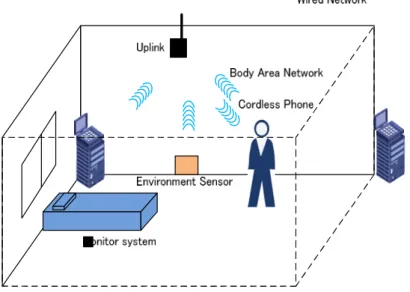
Figure 1 Ultrasonic waves communication system
Today, a wireless communication network is envisioned to provide a wide range of healthcare services. For example, a wireless body area network to capture continuous data from patients in real time [21, 22], or wireless sensor network used in healthcare applications for vital sign collection from medical devices[23].
Figure 1 is an idea diagram of the ultrasonic wireless communication system. A main ultrasonic transceiver is set in every room. This transceiver is used to receive ultrasonic signals sent by other devices and to communicate with other rooms through a wired network. In this system, all the wireless communications use ultrasonic waves. So the remainder of this thesis tests whether ultrasonic waves can be used for an indoor communication system.
1.4 Thesis Layout
The first chapter introduced the background knowledge of this thesis. As wireless communications have been used more and more frequently in our lives, we have found that electromagnetic field waves are not suitable everywhere. So we need something that can be used instead of electromagnetic field waves in some special cases. In this thesis, I chose ultrasonic waves for wireless communication. This is because ultrasonic waves can satisfy some special needs and this has already been used for communication in other areas. This thesis will test whether ultrasonic waves can be used for wireless communication in air, and how it is used.
In Chapter 1, we introduced the background of ultrasonic communication and why we need to use ultrasonic waves for communication.
In Chapter 2, we dealt with the simulation method used for ultrasonic waves. Because there is no suitable simulation method for ultrasonic communication, we introduced a new method in this chapter.
In Chapter 3, we studied a through wall communication system using ultrasonic waves. Experiments were carried out to test this system practically. Both the simulation and the experiment showed that ultrasonic wave is suitable for through-wall communications.
In Chapter 4, we introduced a wireless communication system in the air
using ultrasonic waves. A study of ultrasonic wireless communication in the air has been conducted. Finally, we tested the modulation method used for ultrasonic waves. Compared with other methods, QPSK suited better for this system.
To close, all of these analyses in this thesis proved that ultrasonic waves could be used to build a wireless communication system. Modulated ultrasonic waves can send signals through walls and air. In some special cases, it is better than the traditional electromagnetic field waves.
Chapter 2
Simulation Method for Ultrasonic Communication
2.1 Simulation Method
In order to study a communication system, we need to understand how ultrasonic waves transmit through in the air. The same as electromagnetic field waves, ultrasonic waves will also have reflection and scattering. And both of these will affect wireless communication. So we need a simulation method to study ultrasonic waves. In this chapter we are going to introduce one simulation method.
Indeed, there are almost no simulation methods that can be used for ultrasonic communication now. Generally speaking, most of the simulation methods are used for imaging techniques. For example, the pulse-echo techniques [24,25]. The other ultrasonic simulation method uses the transmitted and reflected energy [26,27]. However, none of these techniques are suitable for ultrasonic communication simulation. This is because they assume that scattering is weak and does not account for strong diffraction and refraction. Therefore, we need another method for the ultrasonic waves simulation.
For the electromagnetic field waves wireless communication, there is a simulation method called the Finite Difference Time Domain(FDTD) method. This is a famous simulation method for electromagnetic simulation.
The FDTD method belongs to the full-wave techniques, which is used to solve electromagnetic problems. Full wave techniques are very useful tools for studying the behavior of the field in any medium. This method uses discrete differences to approximate derivatives in the governing partial differential equations. Because we do not need physical approximations in the FDTD method, it is easy to use. This is an extension used method. For example, it can be used for steady-state simulations, steady-frequency simulations and single-frequency simulations. Another advantage of this method is the cost. When we simulate an N unknowns problem, only N computations are needed. Also, When the complexity and configuration of
the simulation area increase, the increase in the cost is inconspicuous.
When used for electromagnetic simulation, the FDTD method simulates the electromagnetic field in the whole simulation area. For the ultrasonic wave communication, there is an ultrasonic field in the communication area.
So if we can use this method for ultrasonic field simulating, it may become a useful method.
2.2 FDTD Method
2.2.1 Introduction of FDTD Method
In order to use the FDTD method for ultrasonic simulation, we need to understand it first. So I want to introduce the FDTD method in this section.
The FDTD method was first invented in 1966, by Kane Yee[28]. The equations used in his thesis are Maxwell’s curl equations. In his thesis, the simulation area is divided into small cells. Finite difference operators for each magnetic and electric vector were applied. However, Allen Taflove named this method in 1980. After that, the Finite Difference Time Domain method became a famous simulation method[29]. Because of the developments on computer techniques, the FDTD method has become more and more popular for solving problems about electromagnetic field waves since approximately 1990.
When used for simulating electromagnetic field waves, this method uses Maxwell’s differential equations.
D
f
(2.1)0
B
(2.2)E B
t
(2.3)f
H J D
t
(2.4)In the above equations, we can find that the E-field is changed with the H-field in time. Therefore, we can get the value of the E-field of all the
points in the simulation area of the known H-field in the simulation area[28]. The H-field is also the same, and we can update the value of the H-field at all of the simulation area using the same method. This method can be used for two domains, one domain and three-domains. According to Kane Yee’s seminal thesis in 1966, both of the two fields, E and H, can be shown in one unit cell, called the Yee cell.
2.2.2 FDTD Method for Ultrasonic Waves
As mentioned above, the FDTD method simulates the electromagnetic field with Maxwell’s equations. They are a set of partial differential equations which can be used to describe the electromagnetic field. There is also another set of equations for ultrasonic waves. These are called acoustic equations. The same to the E-field and H-field in electromagnetic fields wave, the ultrasonic wave also can write in the form which includes scalar pressure field and the vector velocity. Therefore, the acoustic equations are shown below.
, , 1
2p x y t ( , , )
v x y t
c t
(2.5)
, ,
( , , ) v x y t
xp x y t
x t
(2.6)
, ,
( , , ) v x y ty
p x y t
y t
(2.7)
In the above equations, is the particle velocity, is the sound pressure, and means the density of the tissue. Finally, is the sound speed in the tissue.
To use the FDTD method for ultrasonic simulation, the pressure vector and component vector are discretized in both time and space domains.
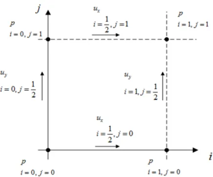
Figure 2 shows the nodes for a 2D ultrasonic FDTD algorithm. We surrounded the velocity components around a pressure node. Therefore, these components are set along the component and the pressure node.
v
p c
Figure 2 Nodes for 2D FDTD method
According to Figure 2, we can change the acoustic wave equations into a finite-difference form and these equations can be used for FDTD simulation.
1/2
1/2
1 2
, 1,
, , (
n n
x x
n n
v i j v i j
p i j p i j t c
x
1/2
,
1/2, 1
n n
y y
v i j v i j
y
(2.8)
1/2 1/2
1, ( , )
, ,
n n
n n
x x
p i j p i j
v i j v i j t
x
(2.9)
1/2 1/2
, 1 ( , )
, ,
n n
n n
y y
p i j p i j v i j v i j t
y
(2.10)2.3 ADI-FDTD Method 2.3.1 Stability Condition
According to the last part, we have one simulation method for ultrasonic waves. However, during the study, I found that the simulation speed is also a big problem. One simulation may take one day or more. So it is necessary to reduce the simulation time. In the FDTD method, we need to divide the simulation area into small cells, and also divide the simulation time into small time steps. Then at each time step, we need to simulate all the cells once. Obviously, the whole simulation will take less time if there are fewer cells or less time steps.
In the traditional FDTD method, simulation errors are also as one of the major limitations. The main reason for the errors is caused by discretizing space[30]. This means that we need enough cells in the simulation area if we want to have a correct result. Because we cannot reduce the volume of space cells, we can only reduce the time step. Yet, for the time step, we have to face another problem. This is the stability condition. The traditional FDTD method should satisfy the stability condition, otherwise the simulation itself will be wrong. The stability condition is shown in the follow equation.
2 2 2
1
1 1 1
t
v x y z
(2.11)
Here, v means the maximum transmit speed in the simulation area. The
x, y and z are the length of the space cell in three directions. This stability condition is called the Courant-Friedrichs-Lewy(CFL) stability condition [31,32]. From this equation, it can be found that the maximum possible length of the time step was limited by the length of the space step.
However, if we need a faster central processing unit compute time in the simulation, we should increase the time step. Therefore, the CFL stability condition will limit the simulation speed. According to equation2.11, in the
CFL condition the minimum space step will limit the possible time step.
These sizes depend on two requirements. The first one is the highest frequency in the simulation. Usually at least 20 cells are needed for one wavelength at the highest frequency. The second one is the structure of the simulation area. All the cells should be smaller than all the objects which are in the simulation area. When the frequency is low, or the object is small, simulation time may become very long. Because the frequency for ultrasonic waves is much lower than electromagnetic field waves, the traditional FDTD method will take a long time for the simulation.
2.3.2 ADI method
In order to increase the simulation speed, a method which can ignore the CFL stability condition appeared. If we do not need to satisfy the CFL stability condition, we can use fewer time steps which means a higher speed. This method was first introduced by Namiki and Zheng. This method is called the Alternating-Direction Implicit(ADI) FDTD method [33-35].
1 2 n
vx pn
1 2 n
vy p vn, nx
, 1 2
n n
x y
v v
1 2
pn
1 2, 1 2
n n
p vy 1
n
vx
1 2
pn 1
n
vy
1, 1 2
n n
x y
v v
1
pn
t
Figure 3Schematic diagram of the ADI-FDTD method
First, the ADI method is used in the research of parabolic equations [31].
As shown in “Alternating-Direction Implicit”, the ADI method will break up each time step. All of these steps will be divided into two smaller time steps. Because this method does not need to follow the CFL condition, any time step can be chosen for one simulation. So the length of the time step will be determined by our requirement but not the condition. This will save a great deal of time in the simulation.
In Figure 3, we showed a schematic diagram of the ADI-FDTD method.
Here, T means time step and Tmax means the maximum time step. Just the same as the ADI-FDTD method used for electromagnetic simulation[36], the simulation step between the nth time step and the (n+1)th time step will be divided into two sub-updating steps. The first sub-updating step is set as the nth to the (n+1/2)th step, as shown in Figure 3. These two procedures will be simulated one by one. Of course, we should spend more time simulating each time step. However, because the number of time steps will be much less than before, the total simulation time will be shorter. Here we have two different ways to solve the ADI-FDTD simulation method. In the first way, n 12
v
x will be updated from
v pxn, n
at first, whereas vxn1 will be updated from
vnx12,pn
in the second updating procedure. In the other way, vny12 will be updated first from
vny, pn
in the first updating procedure, whereasv
ny1will be updated from
vny12,pn
in thesecond step. Generally, the first case is called the x-directional method for the ADI simulation. The other case is called the y-directional ADI simulation method. The calculation processes of these two cases are almost the same. So in this thesis, we choose the first one as the simulation method in this thesis.
2.3.3 Two-Dimensional Equations for ADI Method
The numerical equations of 2-D ultrasonic waves which can be used for the ADI-FDTD method are shown in (2.12)-(17). As mentioned above, two half-steps have been given in these equations. Here, the first half-step is
shown in equations (2.12) -(2.14), while the next half-step is shown in (2.15) -(2.17).
The first:
1
2
1 1
, ,
2 2
n n
x x
v
i j v i j
1 1 1 1
, ,
2 2 2 2 2
n n
t p i j p i j
x
(2.12)
1
2 1 1
, ,
2 2
n n
y y
v i j v i j
1 1
2 1 1 2 1 1
, ,
2 2 2 2 2
n n
t p i j p i j
y
(2.13)
1
2 1 1 1 1
, ,
2 2 2 2
n n
p i j p i j
2
1 1
1, ,
2 2
2
n n
x x
v i j v i j
c t
x
1 1
2 2
2
1 1
, 1 ,
2 2
2
n n
y y
v i j v i j
c t
y
(2.14)
The second:
1
1
1
21
, ,
2 2
n n
x x
v
i j v
i j
1
1 1
11 1
, ,
2 2 2 2 2
n n
t p i j p i j
x
(2.15)1
1
1
21
, ,
2 2
n n
y y
v
i j v
i j
1 1
2 1 1 2 1 1
, ,
2 2 2 2 2
n n
t p i j p i j
y
(2.16)
1
1
1 1
21 1
, ,
2 2 2 2
n n
p
i j p
i j
1 1
2
1 1
1, ,
2 2
2
n n
x x
v i j v i j
c t
x
1 1
2 2
2
1 1
, 1 ,
2 2
2
n n
y y
v i j v i j
c t
y
(2.17)In the first procedure, on the right hand side, both vx component and p component are defined on the nth time step. However, in equation(2.13), the
v
yshown on the left hand side and the pshown on the right hand side are both defined in the (n+1/2)th half-step. Also, the pshown on the left and the vyshown on the right, as shown in equation (2.14), are also defined in the (n+1/2)th half-step. So as shown in (2.13), this equation cannot be used directly for numerical calculation. In order to overcome this problem, equation (2.18) leads from (2.12) and (2.13) by eliminating pn1 2 components. After this, (2.13) can be written in another form using the1 2 n
v
y which forms equation (2.18).1 2 1 1
2 2 2
2 2
1 4 1 1
, 1 2 , , 1
2 2 2
n n n
y y y
v i j y v i j v i j
c t
2
2 2 2
4 1 2 1 1 1 1
, , ,
2 2 2 2 2
n n n
y
y y
v i j p i j p i j
c t c t
1 1
1, ,
2 2
n n
x x
y v i j v i j
x
1 1
1, ,
2 2
n n
x x
y v i j v i j
x
(2.18)
In the first procedure, vy component and pcomponent, which are the right part of equation (2.16), are both defined in the (n+1/2)th half-step.
However, the vx in the left part and the p in the right part of the equation(2.13) are both from the (n+1)th half-step. Also, the pin the left part and the vxin the right part of equation (2.15), are also from the (n+1)th half-step. So in this step, equation (2.15) cannot be used directly for numerical calculation. Here, equation (2.19) leads from (2.15) and (2.17) by eliminating pn1 components. After this, (2.15) can be calculated directly using the vxn1components which are calculated by equation (2.19).
2
1 1 1
2 2
1 4 1 1
1, 2 , 1,
2 2 2
n n n
x x x
v i j x v i j v i j
c t
1 1 1
2
2 2 2
2 2 2
4 1 2 1 1 1 1
, , ,
2 2 2 2 2
n n n
x
x x
v i j p i j p i j
c t c t
1 1
2 1 2 1
, 1 ,
2 2
n n
y y
x v i j v i j
y
1 1
2 1 2 1
, 1 ,
2 2
n n
y y
x v i j v i j
y
(2.19) Both (2.18) and (2.19) are simultaneous linear equations. If we want to solve these equations, we need to write them in the tri-diagonal matrix form.
Then it is very easy to get each vxorvy in the above equations.
2.4 Simulation Test
After the study of the ADI-FDTD method for ultrasonic wave, we want to perform a test by using it. We did two tests here. The first one is a simulation about Gaussian pulse. The second one is the simulation time for both the FDTD method and the ADI-FDTD method.
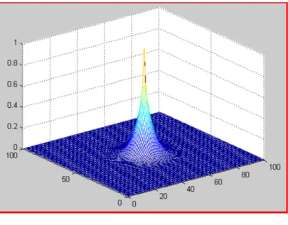
Figure 4 shows a simulation test using the ADI-FDTD method for ultrasonic waves. In this test, the excitation source in the middle of the simulation area is a Gaussian pulse. The simulation area is a square plane, and the length and width are both 5cm. We divide this area into 10,000 cells, so in the figure the length and width are both 100 cells. The vertical axis is normalized amplitude, and the maximum value of the Gaussian pulse is 1. In Figure 5, we simulated the same area as in Figure 4 with a different simulation method. We then compared the simulation times.
(a)
(b)
(c)
Figure 4 Simulation test using the ADI-FDTD method
These three figures show that ultrasonic averagely in the simulation area.
This simulation method works very well in ultrasonic simulation. Then we compared the simulation time for the two FDTD methods. As shown in Figure 5, the simulation time for AID-FDTD is only 1/5 as long as the traditional FDTD when simulating the same area. So in a further study, the ADI-FDTD method will be the simulation method used in this thesis.
FDTD ADI-FDTD 0
20 40 60 80 100
Time[s]
Figure 5 Simulation speed, traditional FDTD and ADI-FDTD
2.4 Conclusion
In this chapter, we dealt with the simulation method used for ultrasonic waves. In order to study a communication system, we first need one simulation method. Therefore, in this chapter, we introduced the background of ultrasonic communication. We dealt with the simulation method used for ultrasonic waves. Because ultrasonic wireless communication is a new area, now there are only a few methods that can be used for simulation. Finally, we chose the FDTD method as the simulation method in my thesis. In the aboriginal FDTD method, simulation errors are one of the major limitations. The other is execution time. The main reasons for the errors are caused by discretizing space and time. Both of them can be calculated from numerical dispersion, and the simulation time is determined by the length of the time step. However, the traditional FDTD method should satisfy the stability condition. Because the frequency of ultrasonic waves is much lower than electromagnetic field waves, the traditional FDTD method may take a long time for the simulation. In order to increase the simulation speed, a method which can ignore CFL stability condition appeared. This method is called the Alternating-Direction Implicit(ADI) FDTD method. This is a new method for ultrasonic simulation, and the theoretical analysis, formula deduction and practical calculation procedures are also presented in this chapter.
Chapter 3
Performance Evaluation of Ultrasonic Communication via Several Medias
3.1 Introduction
In the last chapter, we introduced a new simulation method for ultrasonic wave, the ADI-FDTD method. In order to prove this method can be used for ultrasonic wave simulation, we also tested it by a simple simulation. In that simulation, we simulated a Gaussian pulse in a free space. However, most communication systems use modulated continue waves, and the transmit area is not a free space.
Therefore, in this chapter we want to test whether this method can be used for ultrasonic wave communications’ simulation. This test is divvied into two parts. In the first part, we tested whether the ADI-FDTD method can be used in complex environment. In the second part, we tested whether ADI-FDTD method can be used to simulate modulated continue waves.
Here, a communication system is needed for the simulation. Because the ultrasonic wireless communication in air is a new research area, it is unsuited for this test. We need a well-studied ultrasonic wave communication system. Therefore, we chose through-wall communication to test the simulation method in this chapter.
As mentioned in the first chapter, through wall communication is a main part of ultrasonic communication. We take out both experiments and simulations about the through-wall communication, and compare the result in this chapter. These results will proof whether AID-FDTD method can be used for ultrasonic wave communications’ simulation. After this, we also want to introduce human body communication using ultrasonic waves in this chapter, as this research is similar to through-wall communication. In theory, the ADI-FDTD method can be used for human body simulation, but we need detailed data about the human body if we want to use it. However, we did not have these data, so we mentioned no simulation for human body simulation.
Figure 6 Reflected-pulse method
Before the simulation and experiment, we want to introduce the through-wall communication first. The through-wall communication is very useful today, because there are no useful means for sending digital information across conductive materials, such as metals, water and so on.
Of course, we cannot make holes in these objects every time we need to send data across them. So there is a need for a communication system that can communicate through them.
However, a normal wireless communication system cannot be applied because of the shielding provided by the conductor material, however the ultrasonic waves propagates readily through them and it can also be used to convey information. For example, the use of ultrasonic signaling to transmit digital information across metallic barriers has been demonstrated by several groups[37-41]. Generally speaking, the classic method for though wall communication can be divided into two classes. They are the reflected-pulse approach and the Hybrid approach[42]. First, we want to introduce these two methods.
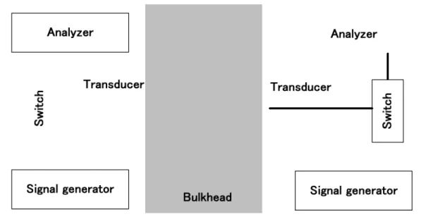
Figure 6 shows the communication system using the reflected pulse method. In this method, only one pair of transducers is needed. The ultrasonic wave source and analyzer are set on the left hand side. On the right hand side, a switch is used as a simple modulator. So in this method, the transducer on the right hand side is considered to be a simple modulator. The amplitude of the reflected wave will be different when we change the electrical load on the right hand side. So binary data can be sent by short circuiting the transducer output for a “0” and open circuiting the transducer output for a “1”.First a pulse will be sent from the left hand side, then the
system on the left hand side will change to receive mode. After the signal comes back, it will be collected by the receive part. The modulator is only set on one side, so this is a one-way transmission system. The data rate will be lower due to the pulse length.
Figure 7 Hybrid method
The next one is the Hybrid method. Because the data rate for the reflected-pulse method is limited by the length of each pulse, in this method, the ultrasonic wave source is changed into a continuous wave source. The diagram of this method is shown in Figure 7. In this method, two transducers are used in the left hand side, and another transducer is used in the right hand side. On the left hand side, the distance between the two transducers is not regular. This system can be used for both pulsed and continuous wave. When a continuous wave carrier is used, the transmit speed will be increased.
However, nowadays two-way communication system is used more often.
So in this chapter, we will use a two-way through wall communication system in the test.
3.2 Simulation for an Ultrasonic Through-Wall System
Figure 8 The schematic diagram of a through-metal ultrasonic system
In this part, we want to introduce the system used. Figure 8 shows the schematic diagram of a through-metal ultrasonic system. In this diagram, we can see that data can be sent by the transducer on either side of this system. Then the signal will come across the bulkhead and be received by the transducer on the other side.
Figure 9 shows the geometry and regions defined for the FDTD simulation. In this simulation, we used three different materials in the simulation area. The transducer is made by steel, the bulkhead is made by aluminium and the rest part is filled by air. Because the sound speed is different in these three materials, ultrasonic wave should reflect on the boundary. So the first simulation is used to test whether the ADI-FDTD method will work in a complex environment. In order to obvious the reflection clearly, we still used a single pulse in this simulation.
The width of the transducer is 3mm and the width of the bulkhead is 4mm. Then we divide this simulation model into square mesh. Each cell of the mesh has its own density and speed of sound. The analysis grid spacing is 0.013mm. So in the simulation, the width of the bulkhead is 307 cells.
Each simulation is running for 20 thousand time steps, for about 3m. These parameters are defined by the sound speed in steel and the frequency of ultrasonic wave, in order to obtaining accurate results.
Bulkhead
Transducer Transducer
Air
Air Air
Air
Figure 9 The geometry defined for the FDTD simulation
The simulation is conducted in an enclosed area, so we need to move it to an open area. In order to do this, we should set absorbing boundaries around the simulation area for this purpose. In this work, we chose the Perfectly Matched Layer(PML) absorber. This technology is a very popular method which is used for the FDTD method[43]. The empty space around the simulation area is the PML absorber. We set the ultrasonic source next to the PML layer on the left hand side transducer. First, we use a Gaussian pulse as the source. As shown in Figure 11(a), this source is a single pulse.
The width of this pulse is about 2000 time steps. In this simulation, each time step means 0.15625ns. So the width of this pulse is 312.5ns. In the other simulation, the length of the time step is the same. In every result, each time step means 0.15625ns.
Figure 10 FDTD simulation, Gaussian pulse propagates in bulkhead
In Figure 10(a), we can see the pulse has entered the bulkhead. Because of the impedance mismatch between the transducer and the bulkhead, only part of the incident energy has been coupled into the bulkhead. Figure 10(b) shows the ultrasonic pulse within the bulkhead.
Figure 10(c) shows that part of the ultrasonic pulse passes into the transducer on the receive side. Again, a portion has been reflected back into the bulkhead. Last, in Figure 10(d), the pulse has been reflected from the receive side of the bulkhead. This part of the pulse will also travel back into the transmitter side. This result shows the performance of ultrasonic wave clearly. The ADI-FDTD method simulated the reflection and the transmission very well. After this, we also want to simulate the received wave form.
-2000 0 2000 4000 6000 8000 10000 12000 14000 16000 18000 0.0
0.2 0.4 0.6 0.8 1.0
-2000 0 2000 4000 6000 8000 10000 12000 14000 16000 18000 -0.3
-0.2 -0.1 0.0 0.1 0.2
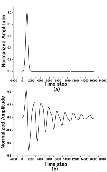
Figure 11 Ultrasonic forces at the transmitter and receiver side
At every step, we measure the acoustic force at both the transmitting transducer side and the receiving transducer side. Figure 11 shows the acoustic force, the figure above is the pulse on the transmitter side and the figure below is the received pulses. Just as the experimental result, a strong primary received pulse is seen, followed by the exponentially decaying series of echo pulses. The primary received pulse corresponds to the transmitted data symbol, and the echoes may cause intersymbol interference with subsequent transmissions.
After the simulation in complex environment, we simulate the modulated continue wave using ADI-FDTD method. First, we will use the Amplitude Shift Keying(ASK) data format. ASK is a simple modulation method. This method sends digital data by changing the amplitude of the carrier waves.
Now this method is widely used in many places.
0 1 2 3 4 5 6 7 8 9 1 0
0 .0 0 .2 0 .4 0 .6 0 .8 1 .0 1 .2
0 5 0 0 0 1 0 0 0 0 1 5 0 0 0 2 0 0 0 0
-1 .0 -0 .5 0 .0 0 .5 1 .0
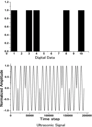
Figure 12 Stochastic data and ASK-modulated signal
In the simulation, we used a group of stochastic data as the source. The
data and the ASK-modulated signal are shown in Figure 12. Data 1 corresponds to 2 cycle of ultrasonic waves, and data 0 corresponds to 2 cycle of zero points.
0 5000 10000 15000 20000
-0.8 -0.6 -0.4 -0.2 0.0 0.2 0.4 0.6 0.8
0 10000 20000 30000 40000
-1.0 -0.5 0.0 0.5 1.0
0 2000 4000 6000 8000 10000 12000 14000 -1.5
-1.0 -0.5 0.0 0.5 1.0 1.5
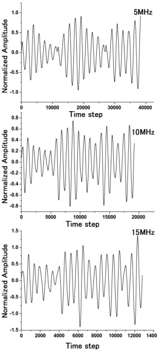
Figure 13 Received signal in different frequency
The simulation area is the same to Figure 10. In this simulation, we only measured the received signal. As previous simulation, we set the source in the left hand part and measure the acoustic force in the right hand part. And
we chose three different frequency for this simulation, they are 5MHz, 10MHz and 15MHz.
In Figure 13, we can see the received signal used a different ultrasonic frequency. Then we compared the received signal with the original signal in Figure 12. From this we observe that the received signal is quite different from the original one. So it will be very hard to set an appropriate threshold value for ASK demodulation. Also, it may also cause transmission errors on the receive side.
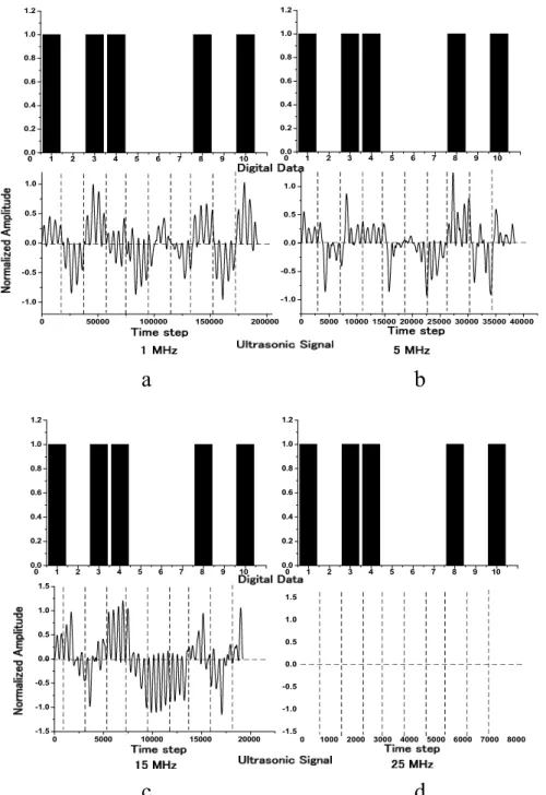
In order to overcome this problem, we tried to use the Binary Phase Keying (BPSK) data format for ultrasonic communication. BPSK is widely used these days in wireless communication networks. This method is particularly well suited in the digital communication area. BPSK can send data much faster than ASK. This method uses two different phases.
So in some case we also call it 2-PSK.The data and the BPSK-modulated signal is shown in Figure 14.
0 1 2 3 4 5 6 7 8 9 10
0.0 0.2 0.4 0.6 0.8 1.0 1.2
0 50000 100000 150000 200000
-1.0 -0.5 0.0 0.5 1.0
Figure 14 Binary Phase Keying data format
In this simulation, we use an aluminum bulkhead, the width of which is 3mm. The same as the ASK simulation, we set the BPSK-modulated signal
180