Pulse Dynamics
of
Reaction-Diffusion
Systems
Shin-Ichiro
Ei
(Yokohama
City
University)
栄伸–郎
(
横浜市立大学
)
joint work withM. Mimura (HiroshimaUniversity)
1
Introduction
In nature, many kinds of spatial $\mathrm{a}\mathrm{n}\mathrm{d}/\mathrm{o}\mathrm{r}$ temporal patterns are observed,
some
of them
are
simple and the others are complicated. To understand theoretically the dynamics of such patterns, many model equations have been proposed and analyzed. Among them, some sort of reaction- diffusion systems are one of the most familarclasses.
Recently, several reaction-diffusion model equations have been known as examples exhibiting various complicated behaviors ofsolutions; self-replicating behaviorofpulses ([6] and its references), refleciton of pulses ([3]), the behavior of pulses like elastic
objects (e.g. [1], [4], [8], [7]).
In this report, we specially consider the particle like dynamics of pulses in two
dimensional space and give a theoretical basis to it.
In [4], following reaction-diffuison systems which has a moving localized solution in two dimensional space was proposed:
(1.1)
where $f(u, v,w)=ru-u^{3}-k_{1}v-k2w$. They showed numerically the existence of a moving localized solution, say travelling spot, under suitable conditions (Fig.1). They
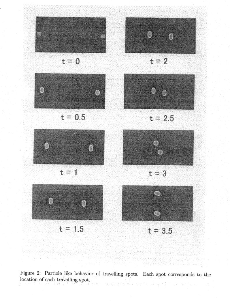
also showed numerically multi travelling spots interact like elastic objects (Fig.2). In order to understand these phenomena, we first consider the existence of a trav-elling spot in two dimensional space under suitable conditions. To show the existence of such moving solutions, we
assume
the existence of stable (radially) symmetricstationary solutions and when it loses the stability, we construct a travelling spot as
the bifurcating solutions from it. ..
Secondly, we analyze their interactions $\dot{\mathrm{w}}\mathrm{h}\mathrm{e}\mathrm{n}$
there exist $\mathrm{m}\mathrm{u}\dot{\mathrm{l}}$
tiple travelling spots.
As a consequence, we can derive ODEs describing the particle like dynamics. The reduced ODEs show how pulses interact and reflection occur.
$\mathrm{u}$
$\mathrm{v}$ $\mathrm{w}$
Figure 1: spatial profiles of atravelling spot. Parameter values are $\epsilon=0.1,$ $\sigma=0.04$, $r=1.5,$ $k_{1}=1.0,$ $k_{2}=5.0,$ $h_{1}=1.0,$ $h_{2}=0.8,$ $\tau=0.01,$ $d=7.\mathrm{o}$
.
2
Construction
of travelling
spot
Let us consider general types of reaction-diffusion systems with bifurcation
param-eter $k$;
.
(2.1) $u_{t}=\mathcal{L}(u;k),$ $x\in R^{2},$ $t>0$,
where $\mathcal{L}(\tau\iota;k)=D\triangle u+F(u;k),$ $u\in R^{N}$ and $D$ is a diagonal matrix with elements
$\{d_{j}\}(j=1,2, \cdots, N)$. We assume following assumptions.
Hl) There exist aradially symmetric standing solution $S(x)$ such that $\mathcal{L}(S(X);k)=0$
and $S(x)arrow 0$ as $|x|arrow\infty$, where $0=(0, \cdots, 0)\in R^{N}$.
Let $X=\{L^{2}(R^{2})\}^{N}$ and let $L(k)=\mathcal{L}’(S(x);k)$ be the linearized operator of (2.1)
with respectto $S(x)$ and$\Sigma(k)$ bethe spectrumof$L(k)$. Note that$L(k)S_{j}=0(j=1,2)$
hold and $0$ is necessarily eigenvalue of$L(k)$, where $S_{j}= \frac{\partial S}{\partial x_{j}}$ for $x=(X_{1}, x_{2})$.
H2) There exists $k=k_{c}$ such that $\Sigma_{c}=\Sigma(k_{c})$ consists of two sets $\Sigma_{0}=\{0\}$ and
$\Sigma_{1}\subset\{z\in C;Re(z)<-\gamma_{0}\}$ for positive constant $\gamma_{0}$. The generalized eigenspace corresponding to $\Sigma_{0}$, say $X_{0}$, is given by $X_{0}--gpan\{sj’\Psi\}j(j=1,2)$, where $\Psi_{j}$ are
functions satisfying $L_{c}\Psi_{j}=-S_{j}(j=1,2)$.
Let $Q_{\mathrm{c}}$ and$R_{c}$ beprojections at $k=k_{c}$ withrespect to $L_{c}$ corresponding to the spectral
sets $\Sigma_{0}$ and $\Sigma_{1}$, respectively. Define a function $U(x;P, \zeta)=S(x-P)+\sum_{j=1}^{2}\zeta_{jj}\Psi$ for $P,$ $\zeta=(\zeta_{1}, \zeta_{2})\in R^{2}$ and a set
At
$=\{S(x-P);P\in R^{2}\}$.We consider (2.1) in the neighborhood ofthe parameter $k=k_{c}$. To do so, we put
$k=k_{c}+\eta$ and rewrite (2.1) as
Figure 2: Particle like behavior of travelling spots. Each spot corresponds to the location of each travalling spot.
where $\mathcal{L}_{c}(u)=\mathcal{L}(u;kc)=D\Delta u+F(u;k_{c})$ and $\eta g(u)=\eta g(u;k)=\mathcal{L}(u;k)-\mathcal{L}_{c}(u)$.
Then, we have the theorem:
Theorem 2.1
If
the initial data $u(\mathrm{O})$ is in the neighborhoodof
$\mathcal{M}$ in $\{H^{2}(R^{2})\}N$,then the solution $u(t)$
of
(2.2)satisfies
$||\mathrm{u}(t)-U(\cdot, P(t),$$\zeta(t))||\infty=o(|\zeta(t)|^{2}+|\eta|)$
as
long as $|\zeta|<\zeta^{*}and|\eta|<\eta^{*}for$constants$\zeta^{*}>0$ and$\eta^{*}>0$. $P$ and$\zeta$ are estimated$by$
$\dot{P}=O(|\zeta(t)|+|\eta|^{2}),\dot{\zeta}=O(|\zeta(t)|^{2}+|\eta|^{2})$.
To obtain more accurate dynamics of $P$ and $\zeta$, we have to know the explicit form of the projection $Q_{\mathrm{c}}$. In fact, the equation governing $P$ and $\zeta$ is formally derived in the similar manner to [2] as
(2.3) $Q_{c^{\frac{d}{dt}U=}}Q_{C}c(U;kC+\eta)+h.O.t.$,
which is in general very difficult to calculate in explicit way.
In the following, we obtain the explicit form of $Q_{c}$ under suitable assumptions and
show the dynamics of$P$ and $\zeta$.
Since the standing solution $S(x)$ is radially symmetric, we write it as $S(x)=S(r)$,
where $r=|x|$. Define the functional space consisting of radially symmetric functions
by $X_{R}=\{L^{2}(0, \infty)\}^{N}$ with the inner product $\langle u, v\rangle_{R}=\int_{0}^{\infty}r\langle u(r), v(r)\rangle dr$ for $u$
and $v\in X_{R}$.
Let $L_{R}(k)$ be the restriction of the linearized operator $L(k)$ on $X_{R}$, that is,
$L_{R}(k)u=D \{u_{rr}+\frac{1}{r}u\}r+F’(S(r);k)u$
for $u\in D_{R}=\{u\in H^{2}(0, \infty)\cap X_{R};u_{r}(0)=0\}$.
H3) The spectrum of $L_{R}(k)$ in $X_{R}$ is uniformly apart from the imaginary axis in the
left hand side for the parameter $k$ in the neighborhood of$k_{c}$.
Define an operator $\overline{L}(k)$ on $X_{R}$ by
$\overline{L}(k)u=D\{u_{r}+\frac{1}{r}u\}_{r}+F’(s(r)7k)u$
for $\mathrm{u}\in\overline{D}=\{u\in H^{2}(0, \infty)\cap X_{R};u(\mathrm{O})=0\}$
.
Here, we note that $\overline{L}(k)s_{r}=-0$ holdswhile $L_{R}(k)S_{r}\neq 0$. This
means
$0$ is necessarily an eigenvalue of $\overline{L}(k)$. Let $L_{c}=\overline{L}(k_{C})$and $\overline{\Sigma}_{c}$ be the spectrum of $\overline{L}_{c}$.
H4) $\overline{\Sigma}_{c}$ consists of two sets $\overline{\Sigma}_{0}=\{0\}$ and $\overline{\Sigma}_{1}\subset\{z\in C;Re\underline{(z})<-\underline{\gamma_{1}}\}$ for a posi-tive constant $\gamma_{1}$. The generalized eigenspace corresponding to
$\overline{X}_{0}=span\{S_{r}, \psi\}$, where $\psi$ is a function satisfying $\overline{L}_{c}\psi=-S_{r}$.
Let $\overline{L}_{c}^{*}$ be the adjoint operator of$\overline{L}_{c}$ in
$X_{R}$
.
Note that it is given by$\overline{L}_{c}^{*}u=D\{u_{r}+\frac{1}{r}u\}_{r}+^{t}F^{;}(S(r);k_{C})u$
.
$\overline{L}_{c}^{*}$ has also similar properties to $\overline{L}_{c}$, that is, there exist eigenfunctions $\phi^{*}$ and $\psi^{*}$ in
$X_{R}$ satisfying $\overline{L}_{c}^{*}\phi^{*}=0$ and $\overline{L}_{c}^{*}\psi*=-\phi^{*}$.
Proposition 2.1 Eigenfunctions $\psi,$ $\phi^{*}$ and $\psi^{*}$ are uniquely determined by the
nor-malization
$\langle\psi, S_{r}\rangle_{R}=\langle\psi, \psi^{*}\rangle R=0,$ $\langle S_{r}, \psi^{*}\rangle_{R}=1$.
We assume eigenfunctions are normalized $\mathrm{a}\mathrm{c}\mathrm{C}\mathrm{o}\mathrm{r}\mathrm{d}\mathrm{i}\mathrm{n}\mathrm{g}^{1}\mathrm{t}\mathrm{o}$ the proposition. Put $\Psi(r)=\int_{0}^{r}\psi(r)dr-\int_{0}^{\infty}\psi(r)dr,$ $\Phi^{*}(r)=\int_{0}^{r_{\emptyset^{*}}}(r)dr-\int_{0}^{\infty}\phi^{*}(r)dr$,
$\Psi^{*}(r)=\int_{0}^{r}\psi^{*}(r)dr-\int_{0}^{\infty}\psi^{*}(r)dr$.
Then, it is easily checked that
$L_{c}\Psi_{j}=-S_{j},$ $L_{cj}^{*}\Phi^{*}=0,$ $L_{c}^{*}\Psi_{j}^{*}=-\Phi_{j}^{*}$
hold for $j=1,2$, where $\Psi_{j}=\frac{\partial\Psi}{\partial x_{j}}$ and so on. By this, we have
Proposition 2.2 The projection$Q_{c}$ is given by
$\pi Q_{\mathrm{c}}u$ $– \int_{0}^{2\pi}\langle u, \phi^{*}\rangle_{R}\cos\theta d\theta\cdot\Psi_{1}+\int_{0}^{2\pi}\langle u, \psi^{*}\rangle_{R}\cos\theta d\theta\cdot s_{1}$
$+ \int_{0}^{2\pi}\langle u, \phi^{*}\rangle_{R}\sin\theta d\theta\cdot\Psi_{2}+\int_{0}^{2\pi}\langle u, \psi^{*}\rangle_{R}\sin\theta d\theta\cdot S_{2}$
for
$u=u(r, \theta)\in X$.By using this expression of $Q_{c}$, we can obtain the explicit dynamics of $P$ and $\zeta$. Theorem 2.2 Under assumptions $Hl$) $-H\mathit{4}$), $P(t)$ and $\zeta(t)$ in theorem 2.1 satisfy
$\{$
$\dot{P}$
$=$ $\zeta+O(|\zeta(t)|^{\mathrm{s}}+|\eta|^{\frac{3}{2})}$,
$\dot{\zeta}$
$=$ $-\nabla W+O(|\zeta(t)|^{4}+|\eta|^{2})$
as long as $|\zeta(t)|<\zeta^{*}$ and $|\eta|<\eta^{*}$, where $W=W( \zeta)=\frac{1}{4}M_{1}|\zeta|^{4}+\frac{1}{2}M_{2}\eta|\zeta|^{2}$
for
Remark 2.1 The values
of
constants $M_{j}$ in Theorem2.2 are
obtainedin explicitforms
while we will not show them in this report, which will be written in [1]. For (1.1), it is numerically checked that both $M_{1}$ and $M_{2}$
are
positive.Remark 2.2 Theorem
2.2
suggests that $\zeta$ denotes the velocityof
the spot$S$ because$P$
denotes the location
of
the spot. $\zeta$ also standsfor
thedeformation
from
radialsymmetryof
spot since the solution $u(t, x)$ is close to thefunction
$U(x;P(t), \zeta(t))$ as in Theorem2.1.
Corollary 2.1 Suppose $M_{1}$ and$M_{2}$
are
positive. $If\eta>0$, there exists astable standingspot with profile $S(x)+O(|\eta|)$ while
if
$\eta<0$, there exists a travelling spot with velocity$(|\zeta(t)|=)\sqrt{\frac{-2M_{2}\eta}{M_{1}}}(1+o(1))$.
3
Interaction
of
two spots
Let us consider how two travelling spots interact.
H5) The standing spot $S(x)$ has an aysmptotic form $S(r) arrow\frac{1}{\sqrt{r}}e^{-\alpha r}a(rarrow\infty)$ for a
constant $\alpha>0$ and a
nonzero
vector $a\in R^{N}$.Remark 3.1 The asymptotic
form
in $H\mathit{5}$) is truefor
many model equations in$R^{2}$
such as the
Gierer-Meinhardt
model ([2]) and the Gray-Scott model ([9]).Define afunction
$U(x;P1, P2, \zeta_{1}, \zeta 2)=\sum_{j=1}\{S(X-Pj)+\langle\zeta j’ x(\nabla\Psi x-P_{j})\rangle\}2$
for $P_{j},$ $\zeta_{j}\in R^{2}$ and define a set
$\mathcal{M}(h^{*})=\{s(x-P1)+S(_{X}-P2);|P_{1}-P_{2}|--h>h^{*}\}$.
Theorem 3.1 There exists a $suffi_{Ciu}eny$ large $h^{*}>0$ such that
if
the initial data $u(\mathrm{O})$is sufficiently close to the set $\mathcal{M}(h^{*})$, then the solution $u.(.t)$
of
(2.2) keeps close to$\dot{U}(x;P_{1,2}P, \zeta_{1}, \zeta_{2})$ with
$u(t)=U(X;P_{1,2}P, \zeta_{1}, \zeta 2)+o(e^{-}\alpha h+|\zeta 1|2|+\zeta 2|2+|\eta|)$
and
for
$j=1,2$(3.1) $\{$
$\dot{P}_{j}$ $=$ $\zeta_{j}\mp M_{0}\frac{1}{\sqrt{h}}e-\alpha he+O(e-2\alpha h+|\zeta 1|\mathrm{s}_{+}|\zeta_{2}|^{\mathrm{s}_{+}\frac{3}{2}}|\eta|)$ ,
$\dot{\zeta}_{j}$ $=$ $- \nabla W(\zeta_{j})\mp\overline{M}0\frac{1}{\sqrt{h}}e^{-\alpha h}e+O(e-2\alpha h+|\zeta 1|4+|\zeta 2|4|+\eta|^{2})$
hold as long as $h>h^{*},$ $|\zeta_{j}(t)|<\zeta^{*}$ and $|\eta|<\eta^{*}$
for
constants $M_{0}$ and $\overline{M}_{0}$, whereRemark 3.2 Constants $M_{0}$ and$\overline{M}_{0}$ are obtained in $e\varphi liCit$way as constants
$M_{1}$ and $M_{2}$ stated in Remark
2.1
while we will not show them in this report, which will bewritten in [1]. For (1.1), it is numerically checked that both $M_{0}$ and$\overline{M}_{0}$ are positive. In the rest of this report, we will intuitively consider the dynamics of$P_{j}$ and $\zeta_{j}$ in thecase of$\eta<0$ (the case of the existence ofa travelling spot). Suppose both $M_{0}$ and
$\overline{M}_{0}$ are positive. To understandthe
dynamics of$\zeta_{j}\mathrm{i}\mathrm{n}\mathrm{t}\mathrm{u}\mathrm{i}- \mathrm{t}\mathrm{i}\mathrm{V}\mathrm{e}\mathrm{l}\mathrm{y}$, weconsider a simplified
ODE
(3.2) $\dot{\zeta}_{1}=-\nabla W(\zeta 1)-Ke$
for a positive constant $K$
.
Since the right hand side of (3.2) is written $\mathrm{b}\mathrm{y}-\nabla W_{1}(\zeta_{1})$,where $W_{1}(\zeta)=W(\zeta)+K\langle\zeta, e\rangle,$ $(3.2)$ has one stable equilibrium with a form $-\beta e$
for $\beta>0$. Thus, $\zeta_{1}$ is pushed toward the direction $\mathrm{o}\mathrm{f}-e$.
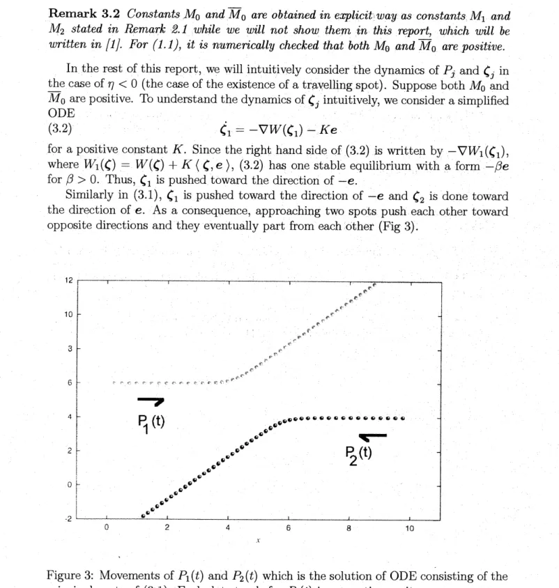
Similarly in (3.1), $\zeta_{1}$ is pushed toward the direction $\mathrm{o}\mathrm{f}-e$ and $\zeta_{2}$ is done toward the direction of $e$. As a consequence, approaching two spots push each other toward
opposite directions and they eventually part from each other (Fig 3).
Figure 3: Movements of$P_{1}(t)$ and $P_{2}(t)$ which is $\dot{\mathrm{t}}$
he solution ofODE consisting of the principal parts of (3.1). Each dot stands for $P_{j}(t)$ in every time unit.
References
[2] S.-I. Ei and J. Wei, Dynamics of
metastable
localized patterns and its applicationtotheinteraction of spike solutions for the
Gierer-Meinhardt
systemsin two spatialdimension, preprint.
[3] S.-I. Ei, M. Mimura and M. Nagayama, Reflection oftravelling pulses in reaction-diffusion systems, in preparation.
[4] S. Kawaguchi and M. Mimura, Collisionof travelling waves in a reaction-diffusion
system with global coupling effect, SIAM J. Appl. Math., 59 (1999),
920-941.
[5] M. Mimura and M. Nagayama, Nonannihilation dynamics in an exothermic
reaction-diffusion system with mono-stable excitability, Chaos 7(4), 1997,
817-826.
[6] Y. Nishiura and D. Ueyama, A skeleton structure of self-replicating dynamics, Physica D, 130 (1999), $7\lambda 104$.
\lceil7\rceil
T. Ohta, Pulse dynamics in a reaction-diffusion system, to appear in Physica D.[8] T. Ohta and T. Ito, Pulse dynamics in an excitable reaction diffusion system,
preprint.
[9] J. Wei, Pattern formation two-dimensional Gray-Scott model: existence of single spot solutions and theirstability, Physica D., to appear.