New scheme for pricing Bermudan options under stochastic volatility model (Mathematical Economics)

New scheme for

pricing Bermudan

options

under

stochastic volatility

model

Masahiro Nishiba

Tokyo

Institute of Technology

2-12-1

Ookayama Meguro-ku

Tokyo

152-8552

Japan

E-mail:

[email protected]

January

30,

2012

Abstract

The author considersstochasticvolatility models and introducesanew

schemefor pricing Bermudan options under stochastic volatility models. Hisapproach is the asymptotic expansion method which is basedon Malli-avin calculus.

1

Introduction

The valuation of Bermudanoptions is veryimportant problem inoption pricing

theory. The values of Bermudan options in stochastic volatility models

are

calculated with the regression method developed by Longstaff and Schwartz [3].

This method is not suitable forparallel computing.

In this paper, we introduce a new scheme for pricing Bermudan options.

This scheme isvery universal and

can

beappliedtoproblems

we can

not develop

recombiningtrees. For example,we canapply to evaluations of derivatives under

SV models.

Our scheme has two keys. One is to derive

an

approximate formula of the

joint distribution function ofstochastic processes using the asymptotic

expan-sion method. The other is to develop recombining treewith the idea of binning

[2] using the approximate joint distribution function. Using the recombining

three, we evaluate derivatives like Bermudanoptions under stochasticvolatility

models. Ourscheme is suitable for parallel computing.

The structure of this paper is

as

follows. The next section reviews the

stochastic volatility models which arewidely accepted infinancial industry and

applies the asymptotic expansion method _{to the model. The 3rd section}

de-scribes how to deriveourapproximateformulaof the joint distributionfunctions

joint distribution function of

SABR

model. The 5th section presents numerical

results of

our

new

scheme. The final section

concludes.

2

Stochastic

volatility

model

2.1

Definition of

stochastic

volatility

model

Let $(\Omega,\mathcal{F},$$\mathbb{P},$ $\{\mathcal{F}_{t}\}_{0\leq t\leq T})$ be

a

complete probability space satisfying the usual

hypotheses and$T\in$ ($0$, oo)denotes

some

fixed horizon of economy. Let $(W_{1}(t), W_{2}(t))$,

$0\leq t\leq T$, be

a

2-dimensional correlated Brownian motion with correlation

given by $\rho:[0, T]arrow[-1,1]$ such that

$d\langle W_{1},$$W_{2}\rangle_{t}=\rho(t)dt$

.

(1)

Weconsider the following stochastic differential equation for X and $Y$:

$dX(t)$ $=$ $B(t, X(t), Y(t))dW_{1}(t)$ , (2)

$dY(t)$ $=$ $M(t, Y(t))dt+D(t, Y(t))dW_{2}(t)$, (3)

$(X$ (0) $, Y(0))$ $=$ $(x_{0}, y_{0})\in \mathbb{R}\cross \mathbb{R}$, (4)

Suppose $B,$ $M$ and $D$ satisfy

some

regularity conditions.

2.2

Asymptotic expansion of

stochastic

volatility

model

We consideran perturbedstochastic process defined

as

the followingstochastic

differential equation:

$dX^{\epsilon}(t)$ $=$ $\epsilon B(t, X^{\epsilon}(t), Y^{\epsilon}(t))dW_{1}(t)$ , (5)

$dY^{\epsilon}(t)$ $=$ $M(t, Y^{\epsilon}(t))dt+\epsilon D(t, Y^{\epsilon}(t))dW_{2}(t)$ , (6)

$(X^{\epsilon}(0), Y^{\epsilon}(0))$ $=$ $(x_{0}, y_{0})\in \mathbb{R}\cross$ R. (7)

We want to calculate

an

approximate solution of this model by using the

asymptotic expansion approach. Byresults of [5], we havethe followinglemma.

Lemma 2.1. $X^{\epsilon}(t)$ and $Y^{\epsilon}(t)$ have following approximate solutions as $\epsilonarrow 0$

respectively.

$X^{\epsilon}(T)$ $=$ $\sum_{i=0}^{N}\epsilon^{i}X_{i}(T)/i!+o(\epsilon^{N})$, (8)

where $X_{i}(T)= \frac{d^{i}X^{\epsilon}(T)}{d\epsilon^{i}}$ $\epsilon=0$ $Y_{i}(T)=\frac{d^{i}Y^{\epsilon}(T)}{d\epsilon^{i}}$ , $\epsilon=0$ (10) (11)

for

$i=0,1,$$\ldots,$$N$

.

Here,

we can

calculate $X_{i}(T)$ and $Y_{i}(T)$ analytically. Examples of $Y_{i}(T)$

are

as

follows:

$Y_{1}^{\epsilon}(T)$ $=$ $\tilde{M}(T)\int_{0}^{T}\tilde{M}(t_{1})^{-1}D(t_{1}, Y_{0}(t_{1}))dW_{2}(t_{1})$ (12)

$Y_{2}^{\epsilon}(T)$ _$=$ $\tilde{M}(T)\int_{0}^{T}\tilde{M}(t_{1})^{-1}Y_{1}(t_{1})^{2}M_{y,y}(t_{1}, Y_{0}(t_{1}))dt_{1}$,

$+$ 2$\tilde{M}(T)\int_{0}^{T}\tilde{M}(t_{1})^{-1}Y_{1}(t_{1})D_{y}(t_{1}, Y_{0}(t_{1}))dW_{2}(t_{1})$ (13)

$Y_{3}^{\epsilon}(T)$ $=$ $\tilde{M}(T)\int_{0}^{T}\tilde{M}(t_{1})^{-1}Y_{1}(t_{1})^{3}M_{y,y,y}(t_{1}, Y_{0}(t_{1}))dt_{1}$ ,

$+$

3

$\tilde{M}(T)\int_{0}^{T}\tilde{M}(t_{1})^{-1}Y_{1}(t_{1})Y_{2}(t_{1})M_{y,y}(t_{1}, Y_{0}(t_{1}))dt_{1}$,

$+$ 3$\overline{M}(T)\int_{0}^{T}\tilde{M}(t_{1})^{-1}Y_{1}(t_{1})^{2}D_{y,y}(t_{1}, Y_{0}(t_{1}))dW_{2}(t_{1})$,

$+$ 3$\tilde{M}(T)\int_{0}^{T}\tilde{M}(t_{1})^{-1}Y_{2}(t_{1})D_{y}(t_{1}, Y_{0}(t_{1}))dW_{2}(t_{1})$ (14)

where

$\tilde{M}(T)$ $=$ $\exp(\int_{0}^{T}M_{y}(t_{0}, Y_{0}(t_{0}))dt_{0})$

.

(15)

And examples

of

$X_{i}(T)$

are

as

follows:

$X_{0}^{\epsilon}(T)$ $=$ $x_{0}$ (17) $X_{1}^{\epsilon}(T)$ $=$ $\int_{0}^{T}B(t_{0}, Y_{0}(t_{0}), X_{0}(t_{0}))dW_{1}(t_{0})$ (18)

$X_{2}^{\epsilon}(T)$ $=$ 2 $\int_{0}^{T}X_{1}(t_{0})B_{y}(t_{0}, Y_{0}(t_{0}), X_{0}(t_{0}))dW_{1}(t_{0})$ (19) $+$ 2 $\int_{0}^{T}Y_{1}(t_{0})B_{x}(t_{0}, Y_{0}(t_{0}), X_{0}(t_{0}))dW_{1}(t_{0})$ (20)

$X_{3}^{\epsilon}(T)$ $=$

3

$\int_{0}^{T}X_{1}(t_{0})^{2}B_{y,y}(t_{0}, Y_{0}(t_{0}), X_{0}(t_{0}))dW_{1}(t_{0})$ (21) $+$ 3 $\int_{0}^{T}X_{2}(t_{0})B_{y}(t_{0}, Y_{0}(t_{0}),X_{0}(t_{0}))dW_{1}(t_{0})$ (22)

$+$ 6 $\int_{0}^{T}X_{1}(t_{0})Y_{1}(t_{0})B_{x,y}(t_{0}, Y_{0}(t_{0}), X_{0}(t_{0}))dW_{1}(t_{0})$ (23)

$+$ 3 $\int_{0}^{T}Y_{1}(t_{0})^{2}B_{x,x}(t_{0}, Y_{0}(t_{0}), X_{0}(t_{0}))dW_{1}(t_{0})$ (24)

$+$ 3 $\int_{0}^{T}Y_{2}(t_{0})B_{x}(t_{0}, Y_{0}(t_{0}), X_{0}(t_{0}))dW_{1}(t_{0})$ (25)

3

Approximation formula of the joint

distribu-tion funcdistribu-tion

We have to calculate conditionalexpectationsto derive

an

approximate formula

ofthe joint distribution function. The next theorem is very useful to calculate

conditional expectations.

Theorem 3.1. Let $f\in L^{2}(T^{n})$

for

$n\geq 1,\dot{d}_{1}\in L(T)$

for

$1\leq j\leq m$

.

Let

$\{W_{i}\}_{i=1,\ldots,n}$ be

an

n-dimensional correlated Brownian motion and $\{Z_{i}\}_{i=1,\ldots,m}$

be

an

m-dimensional correlated Brownian motion. We denote $(t_{1}, t_{2}, \ldots, t_{n})$ by

(t).

$E[\int_{0}^{T}\int_{0}^{t_{1}}\cdots\int_{0}^{t_{\mathfrak{n}-1}}f(t)dW_{n}(t_{n})\cdots dW_{2}(t_{2})dW_{1}(t_{1})|$

$\{\int_{0}^{T}q_{1}^{1}(t)dZ_{1}(t),$_$\ldots,$$\int_{0}^{T}q_{1}^{m}(t)dZ_{m}(t)\}=\{c_{1}, \ldots, c_{m}\}]$

where

$d\langle W_{i},$$Z_{j}\}$ $=$ $\rho_{i,j}dt$, (27)

$\Sigma_{c}$ _$=$ $\{\int_{0}^{T}q_{i}(t)q_{j}(t)dt\}_{i,j=1,\ldots,m}$, (28) $\tilde{\Sigma}(t)$ _$=$ $\{\rho_{i,j}q_{j}(t_{i})\}_{i=1,\ldots,n,j=1,\ldots,m}$ , (29) $\mu(t)$ $=$ $\Sigma_{c}^{-1t_{\Sigma(t)}^{\sim}}$, (30) $\Sigma(t)$ $=$ $-\tilde{\Sigma}(t)\Sigma_{c}^{-1}\tilde{\mathfrak{T}}(t)$, (31)

$m(\xi;\mu(t), \Sigma(t))$ $=$ $\exp(\mu(t){}^{t}\xi+1/2\xi\Sigma(t){}^{t}\xi)$, (32)

$\tilde{H}_{n}(\mu(t), \Sigma(t))$ _$=$ $\frac{d^{n}m(\xi;\mu.(t),\Sigma(t))}{d\xi_{1}\cdot\cdot d\xi_{n}}|_{\xi=0}$

.

(33)

Let $X_{G}^{\epsilon}(T)=(X^{\epsilon}(T)-X_{0}(T))/\epsilon$ and $Y_{G}^{\epsilon}(T)=(\sigma^{\epsilon}(T)-\sigma_{0}(T))/\epsilon$

.

We

want toderivethejointdistribution functionof$X_{G}^{\epsilon}(T)$and$Y_{G}^{\epsilon}(T)$

.

Let_{$\varphi_{X_{G)}Y_{G}}$} :

$\mathbb{R}\cross \mathbb{R}arrow \mathbb{R}$ bea characteristic function of_{$X_{G}^{\epsilon}(T)$} and $Y_{G}^{\epsilon}(T)$

.

Proposition 3.1. $\varphi_{X,Y}$ has an approximate expression

as

follows:

$\varphi_{X_{G},Y_{G}}(\xi_{1}, \xi_{2})$ $=$ $\sum_{i=0}^{N}\frac{\epsilon^{i}}{i!}\frac{d^{i}E[\exp(\sqrt{-1}\xi_{1}X^{\epsilon}(T)+\sqrt{-1}\xi_{2}Y^{\epsilon}(T))]}{d\epsilon^{i}}\epsilon=0+o(\epsilon^{N})$

(34)

for

$(\xi_{1}, \xi_{2})\in \mathbb{R}\cross$R.

In case that $N=2$,

$\varphi_{X_{G},Y_{G}}(\xi_{1}, \xi_{2})$ $=$ $E[N(T)]+\frac{\sqrt{-1}}{2}E[(\xi_{1}X_{2}(T)+\xi_{2}Y_{2}(T))N(T)]$

$+ \frac{\sqrt{-1}\epsilon}{6}E[(\xi_{1}X_{3}(T)+\xi_{2}Y_{3}(T))N(T)]$

$- \frac{\epsilon^{2}}{8}E[(\xi_{1}X_{2}(T)+\xi_{2}Y_{2}(T))^{2}N(T)]+o(\epsilon^{2})$ ₍₃₅₎

where

$N(T)=\exp(\sqrt{-1}\xi_{1}X_{1}(T)+\sqrt{-1}\xi_{2}Y_{1}(T))$ . (36)

By using the inversion formulas of characteristic functions, we get an

approxi-mateformula of the joint probability density function of$X_{G}^{\epsilon}(T)$ and $Y_{G}^{\epsilon}(T)$

.

prob-ability density

_function

$f_{X_{G},Y_{G}}$

as

follows:

$f_{X_{G},Y_{G}}(x,y)$ $=$ $n(x, y; \Sigma)-\frac{1}{2}\frac{d}{dx}\{E^{c}[X_{2}(T)]n(x,y;\Sigma)\}-\frac{1}{2}\frac{d}{dy}\{E^{c}[Y_{2}(T)]n(x,y;\Sigma)\}$

$- \frac{1}{6}\frac{d}{dx}\{E^{c}[X_{3}(T)]n(x,y;\Sigma)\}-\frac{1}{6}\frac{d}{dy}\{E^{c}[Y_{3}(T)]n(x, y;\Sigma)\}$

$+ \frac{1}{8}\frac{d^{2}}{dx^{2}}\{E^{c}[X_{2}(T)^{2}]n(x, y;\Sigma)\}+\frac{1}{8}\frac{d^{2}}{dt^{2}}\{E^{c}[Y_{2}(T)^{2}]n(x,y;\Sigma)\}$

$+ \frac{1}{4}\frac{d^{2}}{dxdy}\{E^{c}[X_{2}(T)n(x, y;\Sigma)]Y_{2}(T)\}$ , (37)

for

$(x, y)\in \mathbb{R}\cross \mathbb{R}$, where

$E^{c}[\cdot]$ $=$ $E[\cdot|(X_{1}(T), Y_{1}(T))=(x, y)]$ , (38)

$n(x,y_{)}\cdot\Sigma)$ $=$ $\frac{1}{2\pi\sqrt{|\Sigma|}}\exp(-[x, y]\Sigma^{-1t}[x,y])$ , (39)

$\Sigma$ _$=$ $[_{E[X_{1}(T)Y_{1}(T)]}E[X_{1}(T)^{2}]$ $E[X_{1}(T)Y_{1}(T)]E[Y_{1}(T)^{2}]]$

.

(40)

Then, $X^{\epsilon}(T)$ and $Y^{\epsilon}(T)$ have a 3rd order $appro\mathfrak{X}mate$joint distribution

func-tion$F_{X,Y}$

as

follows:

$F_{X,Y}(x, y)= \int_{0}^{x-X_{0}(T)}\int_{0}^{y-Y_{0}(T)}f_{X_{G},Y_{G}}(v, w)dwdv$ (41)

We

can

calculateconditional expectationsinthe abovelemma by using

The-orem 3.1.

4

Pricing

Bermudan

options

We introduce

a new

scheme for pricing Bermudan options under stochastic

volatility models in this section. In order to clarify the dependency of the

variables,

we use

notations

as

follows:

$F_{X,Y}(x_{0}, y_{0}, T, x, y)$

$=\mathbb{P}(X(T)\leq x,$$Y(T)\leq y|X(0)=x_{0},$$Y(0)=y_{0})$ . (42)

$\mathbb{P}_{X,Y}(x_{0}, y_{0}, T, l_{x}, u_{x}, l_{y}, u_{y})$

$=\mathbb{P}(l_{x}\leq X(T)\leq u_{x},$$l_{y}\leq Y(T)\leq u_{y}|X(0)=x_{0},$$Y(0)=y_{0})(43)$

We approximate $\mathbb{P}_{X,Y}(x_{0}, y_{0},T, l_{x}, u_{x}, l_{y}, u_{y})$ using results of Section 3. First,

we

have an approximate joint distribution functionof$X$ and $Y$ by Proposition

3.2. Second, we calculate conditional expectations in the approximate joint

distribution function using Theorem 3.1. Thenwehavean approximate formula

4.1

Bermudan

options

Let $T$ be _{$[T_{0}=0, T_{1}, T_{2}, \ldots, T_{n}, \infty]$} for _{$n\geq 1$} and $\mathcal{T}$ be

a

set of stopping time

$\tau$ : $\Omegaarrow$T. We want to calculate avalue $V(t)$ that is defined as follows:

$V(t)$ $=$ $\sup_{\tau\in \mathcal{T}}E[C(\tau, X(\tau), Y(\tau))|\mathcal{F}_{t}]$

.

(44)

Weconsider this option in this section.

4.2

New scheme

Let X be $[x_{1}, x_{2}, \ldots, x_{N}]$ and $Y$ be $[y_{1}, y_{2}, \ldots, y_{M}]$ for $N\geq 1$ and $M\geq 1$

respectively. We define $a_{i}$ for $0\leq i\leq N$ and $b_{j}$ for $0\leq j\leq M$

as

follows:

$a_{i}$ $=$ $\{\begin{array}{ll}-\infty i=0(x_{i}+x_{i+1})/2 i=1,2, \ldots, N-1,\infty i=N\end{array}$ (45)

$b_{i}$ _$=$ $\{\begin{array}{ll}-\infty i=0(x_{i}+x_{i+1})/2 i=1,2, \ldots, M-1.\infty i=M\end{array}$ (46)

We calculate the value$V(k, i,j)$of theoptionat time$T_{k}$ and $(X (T_{k})Y(T_{k}))=$

$(x_{i}, y_{j})$ as follows:

when $k=n$,

$V(k, i,j)$ $=$ $C(T_{k}, x_{i}, y_{j})$, (47)

otherwise,

$V(k, i,j)$ $=$ $\max(C(T_{k}, x_{i}, y_{j}),\sum_{\overline{i}=1,\overline{j}=1}^{N,M}V(k+1,\tilde{t},\tilde{j})\mathbb{P}(i,j, k+1, \tilde{i},\tilde{j}))$ ,

(48)

where

$\mathbb{P}(i,j, k+1,\tilde{i},\tilde{j})=\mathbb{P}(x_{i},$$y_{i},$$T_{k+1}-T_{k},$$a_{\overline{i}-1},$$a_{\overline{i}},$$b_{\overline{j}-1},$$b_{\overline{j}})$

.

(49)

Derivatives

are

valued in this scheme by the usual backwardinductionmethod.

Since a direct construction ofa multidimensional tree would not lead to

recom-bining nodes, thecomputational effort wouldgrownexponentially in thenumber

Table 1: Parameter

$\frac\frac{(i)1000.30.31.00.21.00.01x_{0}y_{0}\alpha\beta\rho\epsilon r}{(ii)1000.30.30.50.2100.01}$

5

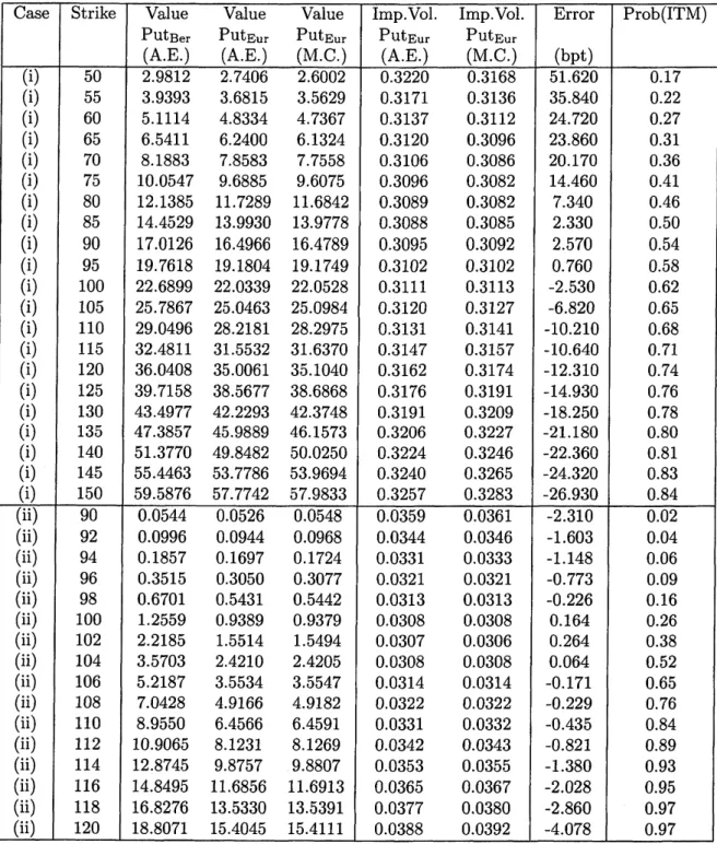
Numerical result

To test the validity of the

new

scheme,

we

consider Bermudan and European

put option under the SABRmodel

as

follows:

$dX^{\epsilon}(t)$ $=$ $\epsilon Y^{\epsilon}(t)X^{\epsilon}(t)^{\beta}dW_{1}(t)$ , (50) $dY^{\epsilon}(t)$ $=$ $\epsilon\alpha Y^{\epsilon}(t)dW_{2}(t)$ , (51)

$d\langle X^{\epsilon},$$Y^{\epsilon}\rangle_{t}$ $=$ $\rho dt$, (52)

$(X^{\epsilon}(0), Y^{\epsilon}(0))$ $=$ $(x_{0}, y_{0})\in \mathbb{R}^{+}\cross \mathbb{R}^{+}$, (53) $S(T)$ $=$ $\exp(rT)X^{\epsilon}(T)$

.

(54)

Let execution times of Bermudan options be $T=\{1.0,2.0$, 3.0,4.0$\}$ and the

maturity ofEuropean option be $T=4.0$

.

We calculate followingvalues.

$Put_{Eur}$ $=$ $E[\exp(-rT)(K-S(T))^{+}]$ , (55)

$Put_{Ber}$ $=$ $\sup_{\tau\in \mathcal{T}}E[\exp(-r\tau)(K-S(\tau))^{+}]$ , (56)

where $\mathcal{T}$ is

a

set ofstopping time

$\tau$ : $\Omegaarrow T$ and $K$ is strike.

In the test ofthe

new

scheme,

we

set $N=100$ and $M=50$, and define$x_{1}$,

$x_{N},$ $y_{1}$ and $y_{M}$

as

follows:

$x_{1}$ $=$ $E[X^{\epsilon}(T)]+5E[(X^{\epsilon}(T)-X_{0}(T))^{2}]^{1/2}$ (57)

$x_{N}$ $=$ $E[X^{\epsilon}(T)]-5E[(X^{\epsilon}(T)-X_{0}(T))^{2}]^{1/2}$ (58) $y_{1}$ $=$ $E[X^{\epsilon}(T)]+5E[(X^{\epsilon}(T)-X_{0}(T))^{2}]^{1/2}$ (59)

$y_{M}$ $=$ $E[Y^{\epsilon}(T)]-5E[(X^{\epsilon}(T)-X_{0}(T))^{2}]^{1/2}$ (60) (61)

The model parameters used in thetest

are

given in Table 1. We

use a

4th order

asymptotic expansion for the joint distribution function and

an

approximate

cumulative bivariate normal probabilities[l].

We

use

values which

are

calculated in Monte Carlo simulations

as

bench-marks. In thesimulations,

we

useNinomiya-Victoir scheme[4]

as a

discretization

scheme with 8 timesteps per

a

year and generate $10^{7}$ paths in each simulation.

Results

are

in Table 2. We compare

our

estimationsof values by

an

A

Proof of Theorem

3.1

A.l

preliminaries

Lemma A.1. Fixed $T\in(0, \infty)$

.

Let $T=[0, T],$ $\mu$ be the Lebesgue measure, $f_{n}\in L^{2}(T^{n}, \sigma(T)^{n}, \mu^{n})$

for

$n\geq 1$ and $(W_{1}, W_{2}, \ldots, W_{n})$ be

a

n-dimensional

correlated Brownian motion. We denote by $\mathcal{E}_{n}$ the set

of

elementary

functions

of

the

_form

$f( t)=\sum_{i_{1},\ldots,i_{n}=1}^{k}c_{i_{1}\cdots i_{n}}1_{A_{:_{1}}\cross\cdots xA_{i_{n}}}(t)$ (62)

where $A_{1},$

$\ldots,$$A_{k}$ are pairwise-disjoint sets belonging to $\sigma(T)$, and the

coeffi-cients $c_{i_{1}\cdots i_{n}}$

are zero

if

any two

of

the indices $i_{1},$ $\ldots,$$i_{n}$

are

equal. Then there

exists a sequence $\{f_{n}^{(l)}\}_{l\in N}\in \mathcal{E}_{n}$ such that $f_{n}^{(l)}\nearrow f_{n}$ and

$E[\int_{0}^{T}\cdots\int_{0}^{T}f_{n}^{(l)}(t)dW_{n}(t_{n})\cdots dW_{1}(t_{1})|\mathcal{G}]arrow$

$E[\int_{0}^{T}\cdots\int_{0}^{T}f_{n}(t)dW_{n}(t_{n})\cdots dW_{1}(t_{1})|\mathcal{G}](a.s.)$ , (63)

where $\mathcal{G}\subset\sigma(T)$

.

A.2

Proof

(64)

We

use

symbols in Lemma A.l. We set $\mathcal{G}$

as

follows:

$\mathcal{G}=\{(\int_{0}^{T}q_{1}^{1}(t)dZ_{1}(t),$

$\ldots,$$\int_{0}^{T}q_{1}^{m}(t)dZ_{m}(t))=(c_{1}, \ldots, c_{m})\}$

.

Then

we

have

$E[\int_{0}^{T}\cdots\int_{0}^{T}f_{n}^{(l)}(t)dW_{n}(t_{n})\cdots dW_{1}(t_{1})|\mathcal{G}]$

$=$ $\sum_{i_{1},\ldots,i_{n}=1}^{k}c_{i_{1}\cdots i_{n}}E[l_{0}^{\tau_{1_{A}}}:_{n}(t)dW_{n}(t)\cdots\int_{0}^{T}1_{A_{1_{1}}}(t)dW_{1}(t)|\mathcal{G}]$

$=$ $l_{0}^{T} \cdots l_{0}^{T}\sum_{i_{1},\ldots,i_{n}=1}^{k}G_{1}\cdots i_{n}1_{A_{:_{1}}\cross\cdots\cross A}:_{n}(t)\hat{H}_{n}(\mu(t), \Sigma(t))dt_{n}\cdots dt_{1}$

$=$ $\int_{0}^{T}\cdots\int_{0}^{T}f_{n}^{(l)}(t)\hat{H}_{n}(\mu(t), \Sigma(t))dt_{n}\cdots dt_{1}$ (65)

We define $f_{n}(t)$

as

follows:

$f_{n}(t)=1_{\{t_{n}\leq\cdots\leq t_{1}\}}(t)f(t)$ , (67)

then

we

have Theorem

3.1.

References

[1] Z. Drezner. Computation of the bivariate normal integral. Mathematics

_of

Computation, $32(141):277-279$, 11978.

[2] Christian P. Fries. Pricing options with early exercise by monte carlo

simu-lation: An introduction. Working Paper, 2005.

[3] Francis A. Longstaff and Eduardo S. Schwartz. Valuing american options

by simulation: A simple least-squares approach. The Review

_of

Financial

Studies, 14:113-147, 2001.

[4] Syoiti Ninomiya and Nicolas Victoir. Weak approximation of stochastic

differential equations and application to derivative pricing. Applied

Mathe-matical Finance, 15:107-121,

2008.

[5] Akihiko Takahashi, Kohta Takehara, and Masashi Toda. Computation in