Home appliances and gender gap of time spent on unpaid housework: Evidence using household data from Vietnam
Tien Manh Vu
Asian Growth Research Institute; and Japan Society for the Promotion of Science
Osaka School of International Public Policy, Osaka University
Working Paper Series Vol. 2016-18 September 2016
The views expressed in this publication are those of the author(s) and do not necessarily reflect those of the Institute.
No part of this article may be used reproduced in any manner whatsoever without written permission except in the case of brief quotations embodied in articles and reviews. For information, please write to the Institute.
Asian Growth Research Institute
Home appliances and gender gap of time spent on unpaid housework: Evidence using household data from Vietnam
Tien Manh Vu 1
Asian Growth Research Institute; and Japan Society for the Promotion of Science
Osaka School of International Public Policy, Osaka University
A BSTRACT We examined the gender gap between wives and husbands with regard to time spent on unpaid housework using interaction terms between the appearance of home appliances and gender among 36,480 Vietnamese households. We found the gender gap is persistent regardless of the number of co-residing children, age cohorts, household size and income, and working status of the couples. In household fixed-effect estimations, the gender gap of time increased with the appearance of home appliances such as gas cookers. One of the main reasons is the reduction in the probability of men participating in housework tasks related to home appliances.
Keywords: home appliances, gender gap, housework, time use, housework division JEL Classification D13, J16, J22
1
Corresponding author: Tien Manh Vu Asian Growth Research Institute
11–4 Otemachi, Kokura–kita, Kitakyushu, Fukuoka 803–0814, JAPAN
Tel +81 93-583-6202 Fax +81 93-583-6576 E–mail: [email protected]
1 Introduction
‘Stoves were labor-saving devices but the labor that they saved was male.’
Cowan (1983: 61) Our study examines whether the gender gap of time spent on unpaid housework exists and whether the appearance of home appliances is associated with a narrower gender gap between husbands and wives in Vietnam. We chose Vietnam because its transitioning economy contains both industrial and agricultural societies. Thanks to trade that is more open and to rising income levels, the lifestyle of Vietnamese households is improving
2. In 2008, approximately 44.6 percent, 11.9 percent, and 31.1 percent of households owned a gas cooker, washing machine, and fridge, respectively
3. However, this implies that the majority of households lived without these appliances. There has also been a shift from agricultural to nonagricultural work. For example, 55.1 percent of workers aged 15 years and over were employed in agriculture, forestry, and fishery in 2005, but this number had fallen to 52.3 percent in 2008
4. Therefore, the allocation of time spent on work, unpaid housework, and leisure has changed while an increase in earnings, according to Becker (1965), would also increase the relative cost of time. In addition, the total fertility rate fell from 2.25 to 2.08 children during 2001–2008
5. Thus, women had an increasing amount of time for paid work, leisure time, and unpaid housework over this period.
There was a rich literature on time use at household level. Along with Mincer (1962), the works of Becker (such as Becker 1965, 1974, 1981, and 1985) would be the foundation for analyses of consumption and time use
6. Blundell, Chiappori, and Meghir (2005); Cherchye, De Rock, and Vermeulen (2012); and Browning, Chiappori and Weiss (2014) are perhaps among the most important extension updates for the collective model of household behavior. Meanwhile, in empirical studies, Hersch (2009) finds that men substitute less paid work for unpaid housework than women do. Gronau (1977) shows that an increase in the wife’s wage rate results in more paid working hours, less housework, and less leisure.
2
Vietnam joined the World Trade Organization in 2006 and experienced average annual GDP growth of over 5 percent from 1990 to 2008
(http://www.gso.gov.vn/default_en.aspx?tabid=468&idmid=3&ItemID=12979).
3
Authors’ calculations.
4
See http://www.gso.gov.vn/default_en.aspx?tabid=467&idmid=3&ItemID=12889.
5
See http://www.gso.gov.vn/default_en.aspx?tabid=467&idmid=3&ItemID=12913.
6
Further history of the development of Becker (1965) can be found Chiappori and Lewbel (2015).
Hersch and Stratton (1994) indicate that the gender gap on unpaid housework is due to the different wage rates of husbands and wives. Wales and Woodland (1997) further estimate the response of housework hours to the ratio of the wage rates. Gough (2011) finds unemployed individuals spend three to seven hours more per week on housework than when employed; and this increase is twice as large for women than for men. However, no empirical study has investigated the case when both do not work, nor addressed the case where couples mix paid work with agricultural work and/or a home business.
Although how husbands and wives allocate time on unpaid housework varies across countries, husbands tend to do less. Ueda (2005) shows that an hour of Japanese husbands’ housework does not perfectly substitute for an hour of wives’ housework. Bloemen, Pasqua, and Stancanelli (2010) find that Italian husbands do less housework. Hersch and Stratton (1994) find that wives employed full time spend more time on both housework and paid work than their husbands do because women earn less. Hersch and Stratton (1994) find that if the gender wage gap declines, time spent on housework will be closer to equal. Folbre and Nelson (2000) find that if wives spend more time on paid work, husbands are less likely to increase time spent on unpaid housework to compensate. However, they did not consider the appearance of home appliances.
The explanations for the reallocation of time between husbands and wives vary and are not simple among empirical studies. Stratton (2012) indicates that men dislike housework. Thus, wives have to compensate. Kroska (2003) reports that women find baby care and laundry-related activities to be
“good, potent, and active” and preparation of meals to be “particularly powerful,” but dislike washing dishes more than men do. Poortman and Lippe (2009) show that women tend to favour cleaning, cooking, and childcare more than men do. Beblo and Robledo (2008) show that husbands have more leisure time because they are Stackelberg leaders in sequential private provision games. Analyzing French workweek reduction policy, Goux, Petrongolo, and Maurin (2014) find that husbands of policy-eligible woman tend to reduce their paid work time, while the wives show little response if their husband was in the target group of the policy.
In this study, we investigate the time of husbands and wives on unpaid housework and paid work
using seemingly unrelated regressions. In the main analysis, we use household fixed-effect models to
estimate the time gap on unpaid housework and then the interaction terms between the appearance of
home appliances and gender. We find the gender gap of time is persistent and around 40.3–58.6 minutes per day, even among dual-nonworking couples. We also find a positive nexus between the appearance of home appliances (gas cooker) and an increase in the time gap indicating less time on unpaid housework for men. We argue that the participation of the husband in specific unpaid housework tasks could be one of the main reasons for this nexus.
Our study extends the previous studies in several ways. To the best of our knowledge, this is the first empirical study analyzing the interaction between home appliances and the gender gap of time spent on unpaid housework. By eliminating the time-invariant factors in household fixed-effect models, we can measure the real “natural” gender gap between husbands and wives. Furthermore, we first consider the interaction terms for more than 26 types of household composition.
2 Data
We use the Vietnamese Household Living Standard Survey 2008 (VHLSS 2008). This provides cross- sectional and country-representative data from the General Statistics Office of Vietnam (GSO) using a two-stage stratified sampling method. The VHLSS 2008 design is identical to the Living Standards Measurement Studies by the World Bank. VHLSS 2008 is the latest survey containing information about housework from 45,945 households comprising 289,948 individuals. In the VHLSS, there are two questions: one about whether individuals do housework and if the answer is yes, the other concerns how many hours per day the individuals spent on housework on average during the previous 12 months.
VHLSS 2008 defines housework as activities such as cleaning, shopping, cooking, washing clothes, fetching water and wood, and repairing tools. We refer to this definition as routine unpaid housework.
The survey includes information about the availability of home appliances such as freezers, vacuum cleaners, washing machines and driers, gas cookers, rice cookers, and microwave ovens.
We use information on time spent on unpaid housework and the presence of home appliances as the main variables. We consider the head and the head’s spouse as the husband and wife of the family in our analysis. After excluding households in which the head does not have a spouse, we have 36,480 households. The descriptive statistics of our data are presented in Tables 1 and 2.
[Insert Tables 1 and 2 here]
3 Empirical methods
We estimate two econometric models. The first are seemingly unrelated regressions (SURs) for the decisions of husbands and wives on time spent on paid work and unpaid housework. The second, put as the main analysis, are household fixed-effect models (HHFEs) for analyzing the gender gap on time spent on unpaid housework.
Learnt the theory for household formation from Phelps (1972), we assume that both husband and wife in a household allocate their time simultaneously between paid work and unpaid housework in four reduced-form SURs as follows.
, (1)
, (2)
,
(3)
. (4)
Each individual is required to consider his/her time spent on paid work and unpaid housework as well as that by their partner. The decision must be based on an individual’s characteristics ( ), their partner’s characteristics ( ) and those of the household ( ). Thus, , , , | with a zero mean across households. Where the couples are not working, the SURs become two equations, (3) and (4).
We use HHFEs to analyze the gender gap in time spent on unpaid housework. For each
household, we assume the time spent on unpaid housework depends mainly on (a) the variation that
covariates with the gender of the individuals, (b) individuals’ characteristics that vary between the
husband and the wife ( ), and (c) the preference or sharing rules or any factors that remain constant
over time within the household ( ).
∗ ∗
∗ (5)
The time-invariant factors are captured by a dummy for each family. We use the Stata command areg in our analysis with 34,679 dummies ( ). Thus, the coefficient shows the “pure”
gender gap in time spent on unpaid housework. Meanwhile, the interactions between the variables of interest with show the marginal gap of time spent on housework between wife and husband if the variables of interest change by one unit, holding all other factors constant within the household.
The main characteristics of individuals are described in Tables 1 and 2. Later labeled Absence–
w/h (Ill day–w/h), “absence” (“ill day”) indicates the total number of days in the 12 months prior to the survey that the wife/husband was absent (ill) and unable to do routine work. We construct four dummies for the number of co-residing children by age cohort from 0–6, 7–12, 13–17, and for couples co-residing without any children.
We also add dummies for the appearance of home appliances in the household as well as construct the first principal component of the six appliances. We notice that pure dual-wage earners are people who work for a salary, but who are not involved in any agricultural work for a family business.
This is done to distinguish them from dual-wage earners who might do both of these types of work.
We divide the data into six main categories as a robustness check of the gender gap, and of the interaction between the variables of interest and gender. These categories are as follows. Working status (both not working, dual-working couples
7, dual-wage earner, and pure dual-wage earner); number of co- residing children (0, 1, 2, 3, 4 and > 4); husband’s age (< 26, 26–35, 36–45, 46–55, 56–65, and > 65);
quartiles of income (4
thquartile is the richest)
8; household size (< 4, 4, 5, and > 5); and dual-chore undertaken couples
9. This is to separate the influence of these categories on the variables of interest and to provide an insight into any differences, if they exist. These categories help us to check the robustness of the results relative to the reduced forms equations of (5).
7
Dual-working couples are those who both do some work for income. Dual-wage earners are those that both do some jobs for wages.
8
This is because the rich have more tools (Cowan 1983).
9
Couples that spent at least one minute on unpaid housework.
In addition, we apply three measures to deal with the high correlations between gas cookers and rice cookers
10/washing machines
11/freezers (0.52, 0.37, and 0.43, respectively). First, we conduct principal component analysis by constructing the first principal component ( ) from six interaction terms between gender and home appliance variables. Second, we retain gas cookers, vacuum cleaners, and microwave ovens in the analyses. Finally, we estimate separately each of the variables of interest for each of the data samples. We test their signs and statistical significance across the various data samples.
We report the analyses with and three appliances as the main results, and present the other results in the Appendix.
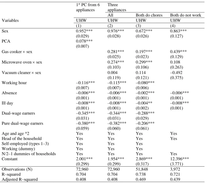
4 Results
As shown in Table 4, the gender gap of time spent on unpaid housework is persistent and approximately 40.3 to 58.6 minutes per day. The gap is 18.24 minutes lower if both the husband and wife do unpaid housework for at least a minute each day. When comparing the gap across the data samples in Table 5, the gaps are statistically significant in 26 samples regardless of the working status, number of co-residing children, birth cohorts, income levels, and household sizes. This is consistent with the results of Vu (2014) who finds a daily 5.25-minute gender gap between Vietnamese siblings aged less than 18 years on daily unpaid housework.
[Insert Tables 3, 4, and 5 here]
We find a substitution between paid work and unpaid housework in Table 3. The rate is different between men and women: 55 (43) minutes of paid work for one hour of unpaid housework for women (men). However, without any paid work, as seen in column (4) of Table 4, the gap is still 52 minutes each day.
Home appliances are associated with different amounts of time spent on housework between husbands and wives. For example, in Table 3, gas cookers help to reduce the time spent on unpaid
10
Unfortunately, the GSO uses the same code for rice cookers, electronic cookers, and pressure cookers.
Therefore, we refer to this variable as “rice cookers” and use the coded variable to construct PCA for the
six variables.
housework for the husbands by much as 1.8 minutes per day. However, gas cookers increase the amount of unpaid housework of wives by 3.8 minutes per day.
The time gap between wives and husbands increases in association with the appearance of home appliances. As shown in column (1) of Table 4, the first principal component of the six home appliances increases the gap by 4.7 minutes per day for wives. We find the estimated is statistically insignificant among pure dual-wage earners, couples with more than four children, husbands aged less than 26, and those in the lowest income quartile as shown in Table 5.
Examining the effects of specific appliances, we find the interaction term constructed from gas cookers and gender has the most statistically significant coefficient of 16.9 minutes per day as shown in column (2) of Table 4. The significance of the coefficients is independent of model specifications that include or exclude other home appliances as shown in the corresponding coefficients in both Table 5 and the Appendix. However, the coefficients become statistically insignificant for pure dual-wage earners where the husband is aged less than 26 years. Among the couples living with more than four children or in the lowest income quartile, the statistically insignificant could be due to the opposite signs of the interaction terms.
The decision to participate in unpaid housework is one of the main reasons for women spending more time on housework following the appearance of gas cookers. We find that with a gas cooker, husbands are 6 percent less likely to do unpaid housework, while the wife is only 0.6 percent less likely as shown in Table 6. This might be because men believe that the cooking with a gas cooker is not difficult enough to warrant their help. Without a gas cooker, men may become involved in tasks such as collecting and chopping firewood.
[Insert Table 6 here]
We hypothesize some additional reasons for the increased gender gap in time associated with the
appearance of home appliances, particularly gas cookers. First, it could be that men do less housework
while women do more, as shown in columns (7) and (8) of Table 3. Second, although gas cookers reduce
cooking time because of convenient heat adjustment and multiple-task heating, they allow women to cook
more dishes per meal. Thus, the total time spent using gas cookers and cleaning dishes (we assume that
women are more likely to do such cleaning) increases. Third, gas cookers might be more closely related
to wives’ tasks, whereas other home appliances could be gender-neutral. Washing machines, microwave ovens, and vacuum cleaners do not require a specific strength or skill related to feminine/masculine characteristics. Fourth, wives could be more involved because they consider cooking time as leisure time.
Indirect evidence is that women who are pure dual-wage earners are more likely to participate (a 1.25 percent increase) if the household owns a gas cooker (see Table 6).
Meanwhile, among pure dual-wage earners, we would argue that the time adjustment of the couples when all income comes from paid work would be rigid. Thus, time constraints give women no opportunity to increase time spent on unpaid housework even if it is considered a leisure activity.
Furthermore, by having stable income, women can have more bargaining power. Thus, men cannot avoid collaborating with women and sharing tasks related to gas cookers. These arguments could explain why the time gap in the two groups is the same, and why women are more likely to do housework where a gas cooker is available.
5 Conclusions and discussion
We examined the time spent on unpaid housework by 36,480 Vietnamese couples. The gender gap is persistent across generations despite changes in the Vietnamese economy. Despite differences in household composition in terms of age, size, income, number of co-residing children, and working status, we found that husbands spend 40.3–58.6 fewer minutes each day on unpaid housework than their wives do. One of the important reasons is that men are less likely to do housework. Working status can explain the substitution between paid work and unpaid housework. However, among dual-nonworking couples, the gender gap of time was still 52 minutes. We also found that some home appliances (such as microwave ovens and gas cookers) reduce the time spent on housework by husbands. Nevertheless, the gender gap of time increases with the appearance of home appliances such as gas cookers. We found that a reduction in the probability of men participating in housework tasks related to gas cookers is one of the main reasons for the larger gap. In addition, a woman may do more housework as a leisure activity and because a gas cooker enables her to cook more dishes and do other related tasks (such as cleaning).
However, this effect does not exist among pure dual-wage earners or in cases where husbands are aged
less than 26 years.
We acknowledge several limitations of our data and analyses. First, the time spent on housework is retrospective, but not in a form of time use survey where each specific task of each individual is recorded with both the starting and the ending time. Second, we bypassed the self-selection of men and women toward specific tasks, the productivity of doing housework and the collaboration between couples on the same task. Thus, the gender gap might be associated with the specific tasks included in the survey.
Third, we were only able to consider gas cookers, but not other types of cookers such as electronic cookers, pressure cookers, and rice cookers. This is because the survey coded the three mentioned cookers in the same variable.
The positive relationship between gender gap of time and the appearance of home appliances has several policy implications. First, the gap exists because individuals might be self-selected to certain specific tasks of unpaid housework. Thus, policies to increase the participation of women in paid work should consider this effect. Second, the positive interaction terms indicate that the policies facilitating the participation of men in housework also empower women. This can also influence the marketing strategies of the suppliers of home appliances. Similarly, policies aimed at empowering women via microcredit should consider this interaction. Finally, our study confirms the existence of gender roles in terms of unpaid housework between husbands and wives.
Acknowledgments We thank Hisakazu Matsushige, Charles Yuji Horioka, Euston Quah, Yoko Niimi and the participants of the International Association for Feminist Economics Annual Conference held in Berlin, Germany, in July 2015 and of the Asian Consumer and Family Economics Association held in Hong Kong Shue Yan University, Hong Kong, in July 2016 for the valuable comments and suggestions.
We acknowledge the financial support from the JSPS KAKENHI Grant number A26043110 from the Japanese Society for the Promotion of Science.
References
Beblo, M. and J.R. Robledo (2008). The wage gap and the leisure gap for double-earner couples. Journal of Population Economics, 21(2), pp. 281–304.
Becker, G. S (1965). A theory of allocation of time. The Economic Journal, 75, pp. 493–517.
Becker, G. S (1974). A theory of social interactions. Journal of Political Economy, 82, pp. 1063–1093.
Becker, G. S (1981). A treatise on the family. Cambridge, MA: Havard University Press.
Becker, G. S (1985). Human capital, effort, and the sexual division of labor. Journal of Labor Economics,
3(1), pp. S33–S58.
Bloemen, H. G., Pasqua, S., and E.G F. Stancanelli (2010). An empirical analysis of the time allocation of Italian couples: are they responsive? Review of Economics of the Household, 8(3), pp. 345–369.
Blundell, R., Chiappori, P.A, and C. Meghir (2005). Collective labor supply with children. Journal of Political Economy, 113, pp. 1277–1306.
Browning, M., Chiappori, P. A., and Y. Weiss (2014). Economics of the Family. Cambridge University Press, Cambridge.
Cherchye, L., De Rock, B., and F. Vermeulen (2012). Married with children: a collective labor supply model with detailed time use and intrahousehold expenditure information. American Economic Review, 102, pp. 3377–3405.
Chiappori, P. A., and A. Lewbel (2015). Gary Becker's a theory of the allocation of time. The Economic Journal, 125, pp. 410–442.
Cowan, R. S (1983). More work for mother. Basic Books, New York.
Folbre, N., and J.A. Nelson (2000). For love or money—or both? Journal of Economic Perspectives, 14(4), pp. 123–140.
Gough, M (2011). Unemployment in families: The case of housework. The Journal of Industrial Economics, 59(3), pp. 1085–1100.
Goux, D., Petrongolo, B. and E. Maurin (2014). Worktime regulations and spousal labor supply.
American Economic Review, 104(5639), pp. 252–276.
Gronau, R (1977). Leisure, home production, and work––the theory of the allocation of time revisited.
Journal of Political Economy, 85(6), pp. 1099
Hersch, J (2009). Home production and wages: Evidence from the American Time Use Survey. Review of Economics of the Household, 7(2), pp. 159–178.
Hersch, J. and L.S. Stratton (1994). Housework, wages, and the division of housework time for employed spouses. American Economic Review, 84(2), pp. 120–125.
Hersch, J. and L.S. Stratton (1997). Housework, fixed effects, and wages of married workers. Journal of Human Resources, 32(2), pp. 285–307.
Kroska, A (2003). Investigating gender differences in the meaning of household chores and child care.
Journal of Marriage and Family, 65(2), pp. 456–473.
Mincer, J (1962). Labor force participation of married women: a study of labor supply. In H. G. Lewis (Ed.), Aspects of Labor Economics (pp. 63–105). Princeton, N.J.: Princeton University Press.
Phelps, C. D (1972). Is the household obsolete? American Economic Review, 62(1–2), pp. 167–174.
Poortman, A. R. and T.V.D. Lippe (2009). Attitudes toward housework and child care and the gendered division of labor. Journal of Marriage and Family, 71(3), pp. 526–541.
Stratton, L. S (2012). The role of preferences and opportunity costs in determining the time allocated to housework. American Economic Review, 102(3), pp. 606–611.
Ueda, A (2005). Intrafamily time allocation of housework: Evidence from Japan. Journal of the Japanese and International Economies, 19(1), pp. 1–23.
Vu, T. M (2014). Are daughters always the losers in the chore war? Evidence using household data from Vietnam. Journal of Development Studies, 50(4), pp. 520–529.
Wales, T. J. and A.D. Woodland (1977). Estimation of the allocation of time for work, leisure, and
housework. Econometrica, 45(1), pp. 115–132.
Appendix Robustness checks by separating each home appliance per estimation and by data sample
Data selections N Interaction between sex and Gas cooker Std. err.
Microwave
oven Std. err.
Vacuum
cleaner Std. err. Freezer Std. err.
Washing
machine Std. err.
Rice
cooker Std. err.
All (1) 72,960 0.295*** (0.025) 0.399*** (0.097) 0.224** (0.113) 0.244*** (0.028) 0.326*** (0.044) 0.138*** (0.025) Dual-nonworking (2) 3,972 0.434*** (0.127) 0.142 (0.249) –0.348 (0.353) 0.358*** (0.127) 0.328** (0.152) 0.289* (0.151) Dual-working (3) 60,506 0.218*** (0.024) 0.383*** (0.113) 0.349*** (0.121) 0.181*** (0.027) 0.291*** (0.046) 0.107*** (0.024) Dual-wage earner (4) 12,120 0.158*** (0.054) 0.169 (0.205) 0.408** (0.201) 0.149** (0.062) 0.161* (0.084) 0.063 (0.056) Pure dual-wage earner (5) 4,642 0.058 (0.104) 0.001 (0.222) 0.421* (0.230) 0.091 (0.099) 0.024 (0.106) 0.051 (0.123) Living without a child (6) 7,708 0.165** (0.073) 0.579** (0.286) 0.125 (0.240) 0.203** (0.084) 0.357** (0.175) –0.003 (0.077) 1 child
a(7) 15,366 0.254*** (0.054) 0.383* (0.219) 0.242 (0.259) 0.197*** (0.060) 0.263*** (0.094) 0.094* (0.056) 2 children (8) 29,734 0.318*** (0.037) 0.335** (0.135) 0.273 (0.170) 0.237*** (0.040) 0.306*** (0.057) 0.158*** (0.039) 3 children (9) 12,916 0.341*** (0.064) 0.567** (0.223) 0.213 (0.234) 0.358*** (0.072) 0.431*** (0.121) 0.173*** (0.061) 4 children (10) 4,664 0.264** (0.103) 0.539 (0.545) 0.039 (0.541) 0.100 (0.130) 0.442* (0.245) 0.192** (0.093) More than 4 children (11) 2,572 0.326** (0.162) –0.933 (0.580) –1.073 (1.107) 0.221 (0.188) –0.027 (0.362) 0.376*** (0.133)
Husband age < 26 (12) 576 0.143 (0.365) 0.474 (0.441) 0.482 (0.833) 0.411 (0.260)
Husband age 26–35 (13) 9,308 0.268*** (0.068) –0.065 (0.356) 0.220 (0.369) 0.155* (0.083) 0.044 (0.126) 0.153** (0.065)
Husband age 36–45 (14) 23,292 0.243*** (0.042) 0.241 (0.233) 0.256 (0.212) 0.199*** (0.048) 0.227*** (0.078) 0.156*** (0.042)
Husband age 46–55 (15) 21,686 0.308*** (0.044) 0.445*** (0.135) 0.377** (0.160) 0.237*** (0.047) 0.385*** (0.073) 0.135*** (0.047)
Husband age 56–65 (16) 10,192 0.333*** (0.065) 0.477** (0.228) –0.075 (0.267) 0.349*** (0.073) 0.544*** (0.108) 0.116* (0.070)
Husband age > 65 (17) 7,906 0.302*** (0.081) 0.556** (0.250) 0.274 (0.410) 0.252*** (0.091) 0.252* (0.146) 0.056 (0.083)
1
stquartile income (18) 18,236 0.190*** (0.073) –0.711 (1.147) 0.217 (0.400) 0.023 (0.112) –0.166 (0.278) 0.051 (0.043)
2
ndquartile income (19) 18,238 0.224*** (0.047) 0.182 (0.418) –0.227 (0.389) 0.008 (0.062) 0.061 (0.190) 0.024 (0.045)
3
rdquartile income (20) 18,252 0.174*** (0.048) 0.556** (0.270) 0.008 (0.300) 0.091* (0.051) 0.203** (0.089) 0.040 (0.061)
4
thquartile income (21) 18,234 0.267*** (0.064) 0.233** (0.107) 0.112 (0.132) 0.269*** (0.055) 0.224*** (0.058) 0.050 (0.084)
Household size <4 (22) 18,408 0.208*** (0.049) 0.304 (0.209) 0.124 (0.216) 0.183*** (0.056) 0.240** (0.096) 0.033 (0.050)
Household size = 4 (23) 24,990 0.288*** (0.040) 0.494*** (0.141) 0.393** (0.188) 0.242*** (0.044) 0.323*** (0.063) 0.154*** (0.044)
Household size = 5 (24) 15,138 0.345*** (0.054) 0.457** (0.228) 0.206 (0.246) 0.291*** (0.060) 0.391*** (0.099) 0.167*** (0.052)
Household size > 5 (25) 14,424 0.347*** (0.060) 0.272 (0.224) 0.034 (0.275) 0.251*** (0.068) 0.340*** (0.112) 0.205*** (0.056)
Dual chore undertaken (26) 51,848 0.214*** (0.023) 0.413*** (0.100) 0.306*** (0.116) 0.205*** (0.027) 0.299*** (0.044) 0.142*** (0.022)
Notes:
aChildren are those of the head and are co-residing in the household. Other control variables are the same as in Table 4
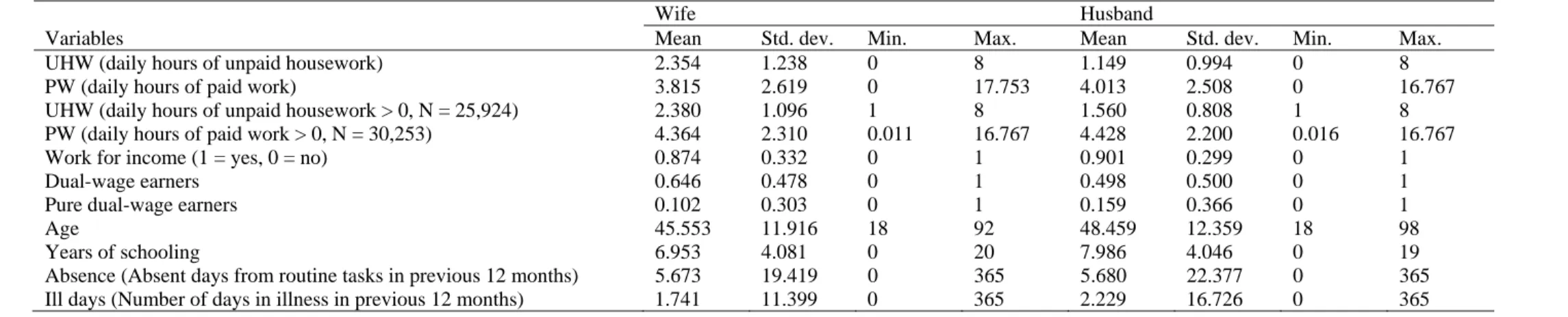
Table 1 Descriptive statistics of husbands and wives in the selected sample
Wife Husband
Variables Mean Std. dev. Min. Max. Mean Std. dev. Min. Max.
UHW (daily hours of unpaid housework) 2.354 1.238 0 8 1.149 0.994 0 8
PW (daily hours of paid work) 3.815 2.619 0 17.753 4.013 2.508 0 16.767
UHW (daily hours of unpaid housework > 0, N = 25,924) 2.380 1.096 1 8 1.560 0.808 1 8 PW (daily hours of paid work > 0, N = 30,253) 4.364 2.310 0.011 16.767 4.428 2.200 0.016 16.767
Work for income (1 = yes, 0 = no) 0.874 0.332 0 1 0.901 0.299 0 1
Dual-wage earners 0.646 0.478 0 1 0.498 0.500 0 1
Pure dual-wage earners 0.102 0.303 0 1 0.159 0.366 0 1
Age 45.553 11.916 18 92 48.459 12.359 18 98
Years of schooling 6.953 4.081 0 20 7.986 4.046 0 19
Absence (Absent days from routine tasks in previous 12 months) 5.673 19.419 0 365 5.680 22.377 0 365
Ill days (Number of days in illness in previous 12 months) 1.741 11.399 0 365 2.229 16.726 0 365
Note: Total number of households = 36,480
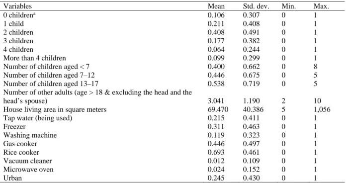
Table 2 Descriptive statistics of households in the selected sample
Variables Mean Std. dev. Min. Max.
0 children
a0.106 0.307 0 1
1 child 0.211 0.408 0 1
2 children 0.408 0.491 0 1
3 children 0.177 0.382 0 1
4 children 0.064 0.244 0 1
More than 4 children 0.099 0.299 0 1
Number of children aged < 7 0.400 0.662 0 8
Number of children aged 7–12 0.446 0.675 0 5
Number of children aged 13–17 0.538 0.719 0 5
Number of other adults (age > 18 & excluding the head and the
head’s spouse) 3.041 1.190 2 10
House living area in square meters 69.470 40.386 5 1,056
Tap water (being used) 0.215 0.411 0 1
Freezer 0.311 0.463 0 1
Washing machine 0.119 0.323 0 1
Gas cooker 0.446 0.497 0 1
Rice cooker 0.693 0.461 0 1
Vacuum cleaner 0.012 0.109 0 1
Microwave oven 0.024 0.152 0 1
Urban 0.245 0.430 0 1
Notes:
aChildren are those of the head and are co-residing in the household. Total number of households =
36,480
Table 3 Seemingly unrelated regressions with four decisions on time spent on paid work and
unpaid housework
1
stPC of 6 appliances Three appliances
Variables PW–w PW–h UHW–w UHW–h PW–w PW–h UHW–w UHW–h
(1) (2) (3) (4) (5) (6) (7) (8)
PW–w
0.601***–
0.263*** 0.144*** 0.601*** –0.263*** 0.144***(0.004) (0.003) (0.002) (0.004) (0.003) (0.002)
PW–h
0.681*** 0.191*** –0.158*** 0.681*** 0.190*** –0.158***(0.005) (0.003) (0.002) (0.005) (0.003) (0.002)
UHW–w
–0.913*** 0.636*** 0.246*** –0.913*** 0.636*** 0.246***(0.009) (0.009) (0.004) (0.009) (0.009) (0.004)
UHW–h
0.746*** –0.721*** 0.347*** 0.746*** –0.721*** 0.347***(0.012) (0.011) (0.006) (0.012) (0.011) (0.006)
Absence–w
–0.010*** –0.005*** 0.003*** –0.010*** –0.005*** 0.003***(0.001) (0.000) (0.000) (0.001) (0.000) (0.000)
Ill day–w
–0.010*** –0.007*** 0.005*** –0.010*** –0.007*** 0.005***(0.001) (0.001) (0.000) (0.001) (0.001) (0.000)
Absence–h
–0.010*** 0.002*** –0.003*** –0.010*** 0.002*** –0.003***(0.000) (0.000) (0.000) (0.000) (0.000) (0.000)
Ill day–h
–0.008*** 0.003*** –0.004*** –0.008*** 0.003*** –0.004***(0.001) (0.000) (0.000) (0.001) (0.000) (0.000)
Living without a child
0.023 0.088*** 0.022 0.089***(0.023) (0.020) (0.023) (0.020)
Child
aaged < 7
0.011 0.002 0.012 0.001(0.010) (0.008) (0.010) (0.008)
Child aged 7–12
–0.029*** –0.019** –0.028*** –0.019**(0.009) (0.008) (0.009) (0.008)
Child aged 13–17
–0.070*** –0.074*** –0.069*** –0.074***(0.009) (0.008) (0.009) (0.008)
Number of adults
–0.056*** –0.073*** –0.056*** –0.073***(0.006) (0.005) (0.006) (0.005)
House living area
0.000*** –0.000 0.000*** –0.000*(0.000) (0.000) (0.000) (0.000)
Tap water
0.041** –0.045*** 0.042** –0.047***(0.018) (0.015) (0.018) (0.015)
PCA (6 appliances)
0.015*** –0.014***(0.005) (0.004)
Gas cooker
0.063*** –0.030**(0.014) (0.012)
Vacuum cleaner
0.002 –0.031(0.055) (0.047)
Microwave oven
–0.006 –0.067*(0.041) (0.035)
Age and age ^2
Yes Yes Yes Yes Yes Yes Yes YesSchooling years
Yes Yes Yes YesProvinces & urban
Yes Yes Yes YesConstant
0.631*** 1.403*** 1.967*** 0.632*** 0.630*** 1.405*** 1.943*** 0.656***(0.144) (0.148) (0.090) (0.083) (0.144) (0.148) (0.090) (0.083)
Observations 36,480 36,480 36,480 36,480 36,480 36,480 36,480 36,480
R–squared 0.182 0.239 0.107 0.040 0.182 0.239 0.108 0.040
Notes: Robust standard errors in parentheses (*** p < 0.01, ** p < 0.05, * p < 0.1). Children are those of the
head and are coresiding in the household
Table 4 Household fixed-effect models on time spent on unpaid housework
1
stPC from 6 appliances
Three
appliances
All Both do chores Both do not work
Variables UHW UHW UHW UHW
(1) (2) (3) (4)
Sex 0.952*** 0.976*** 0.672*** 0.863***
(0.029) (0.028) (0.026) (0.127)
PCA 0.078***
(0.007)
Gas cooker sex 0.281*** 0.197*** 0.439***
(0.025) (0.023) (0.129)
Microwave oven sex 0.274*** 0.299*** 0.108
(0.103) (0.106) (0.263)
Vacuum cleaner sex 0.004 0.114 –0.492
(0.119) (0.121) (0.375)
Working hour –0.116*** –0.115*** –0.080***
(0.007) (0.007) (0.006)
Absence –0.006*** –0.006*** –0.002*** –0.006***
(0.001) (0.001) (0.001) (0.001)
Ill day –0.008*** –0.008*** –0.004** –0.008***
(0.001) (0.001) (0.002) (0.001)
Dual-wage earners –0.345*** –0.344*** –0.288***
(0.031) (0.031) (0.029)
Pure dual-wage earners –0.380*** –0.382*** –0.206***
(0.059) (0.060) (0.061)
Age and age ^2 Yes Yes Yes Yes
Head of the household Yes Yes Yes Yes
Self-employed (types 1–3) Yes Yes Yes
Working (dummy) Yes Yes Yes
N/2–1 dummies of households Yes Yes Yes Yes
Constant 2.001*** 1.954*** 2.869*** 12.396***
(0.299) (0.299) (0.317) (3.771)
Observations (N) 72,960 72,960 51,848 3,972
R–squared 0.704 0.704 0.738 0.721
Adjusted R–squared 0.408 0.408 0.469 0.439
Note: Robust standard errors in parentheses (*** p < 0.01, ** p < 0.05, * p < 0.1)
Table 5 Interaction terms by data sample
Data selections N 1
stPC from 6 appliances Three appliances Sex St. err. PCA St. err. Sex St. err.
Gas cooker
sex St. err.
Microwave
sex St. err.
Vacuum
sex St. err.
All (1) 72,960 0.952*** (0.029) 0.078*** (0.007) 0.976*** (0.028) 0.281*** (0.025) 0.274*** (0.103) 0.004 (0.119) Dual-nonworking (2) 3,972 0.874*** (0.136) 0.101*** (0.036) 0.863*** (0.127) 0.439*** (0.129) 0.108 (0.263) –0.492 (0.375) Dual-working (3) 60,506 0.881*** (0.030) 0.062*** (0.007) 0.910*** (0.029) 0.204*** (0.024) 0.250** (0.120) 0.172 (0.127) Dual-wage earner (4) 12,120 1.001*** (0.060) 0.043*** (0.016) 1.013*** (0.057) 0.145*** (0.054) 0.010 (0.234) 0.347 (0.241) Pure dual-wage earner (5) 4,642 1.149*** (0.112) 0.026 (0.031) 1.179*** (0.105) 0.051 (0.105) –0.150 (0.251) 0.498* (0.276) Living without a child (6) 7,708 0.803*** (0.077) 0.060*** (0.021) 0.848*** (0.076) 0.143* (0.074) 0.526* (0.302) –0.089 (0.245) 1 child
a(7) 15,366 0.978*** (0.061) 0.066*** (0.017) 0.992*** (0.056) 0.236*** (0.054) 0.274 (0.233) 0.042 (0.269) 2 children (8) 29,734 0.918*** (0.044) 0.083*** (0.011) 0.939*** (0.042) 0.306*** (0.037) 0.195 (0.143) 0.086 (0.178) 3 children (9) 12,916 1.025*** (0.088) 0.096*** (0.017) 1.079*** (0.090) 0.324*** (0.064) 0.448* (0.240) –0.096 (0.264) 4 children (10) 4,664 1.094*** (0.129) 0.066** (0.030) 1.105*** (0.123) 0.251** (0.102) 0.501 (0.607) –0.366 (0.679)
> 4 children (11) 2,572 1.210*** (0.167) 0.033 (0.039) 1.140*** (0.162) 0.363** (0.163) –1.069 (0.680) –0.229 (1.230) Husband aged < 26 (12) 576 1.033*** (0.368) 0.081 (0.065) 1.120*** (0.377) 0.143 (0.365)
Husband aged 26–35 (13) 9,308 0.949*** (0.087) 0.040** (0.018) 0.910*** (0.084) 0.273*** (0.069) –0.266 (0.341) 0.191 (0.362)
Husband aged 36–45 (14) 23,292 0.990*** (0.054) 0.062*** (0.013) 1.010*** (0.053) 0.236*** (0.042) 0.109 (0.263) 0.126 (0.249)
Husband aged 46–55 (15) 21,686 0.952*** (0.049) 0.090*** (0.012) 0.994*** (0.047) 0.287*** (0.044) 0.291** (0.144) 0.156 (0.170)
Husband aged 56–65 (16) 10,192 0.853*** (0.077) 0.105*** (0.020) 0.918*** (0.071) 0.314*** (0.066) 0.410* (0.238) –0.350 (0.283)
Husband aged > 65 (17) 7,906 0.799*** (0.095) 0.072*** (0.022) 0.805*** (0.093) 0.272*** (0.082) 0.437* (0.254) –0.017 (0.408)
1
stquartile income (18) 18,236 0.855*** (0.064) 0.017 (0.014) 0.849*** (0.063) 0.194*** (0.073) –0.855 (1.149) 0.237 (0.436)
2
ndquartile income (19) 18,238 0.967*** (0.055) 0.033** (0.014) 0.949*** (0.052) 0.224*** (0.047) 0.118 (0.425) –0.266 (0.378)
3
rdquartile income (20) 18,252 1.056*** (0.062) 0.055*** (0.016) 1.081*** (0.057) 0.169*** (0.048) 0.511* (0.265) –0.096 (0.307)
4
thquartile income (21) 18,234 0.970*** (0.071) 0.096*** (0.019) 1.041*** (0.069) 0.249*** (0.065) 0.198* (0.115) –0.010 (0.141)
Household size < 4 (22) 18,408 0.917*** (0.054) 0.054*** (0.015) 0.927*** (0.050) 0.197*** (0.049) 0.224 (0.222) –0.030 (0.228)
Household size = 4 (23) 24,990 0.930*** (0.048) 0.086*** (0.011) 0.971*** (0.046) 0.267*** (0.041) 0.351** (0.150) 0.165 (0.196)
Household size = 5 (24) 15,138 0.969*** (0.069) 0.090*** (0.015) 1.004*** (0.071) 0.333*** (0.055) 0.328 (0.241) –0.048 (0.257)
Household size > 5 (25) 14,424 1.048*** (0.078) 0.072*** (0.016) 1.047*** (0.074) 0.343*** (0.060) 0.161 (0.244) –0.209 (0.303)
Dual chore undertaken (26) 51,848 0.630*** (0.027) 0.067*** (0.007) 0.672*** (0.026) 0.197*** (0.023) 0.299*** (0.106) 0.114 (0.121)
Table 6 Mean comparison tests between two samples, with and without gas cooker
Data selections Gas cooker available (A) Without gas cooker (B) Difference
Obs. Mean Obs. Mean (A)–(B)
All
Participation–H
a16,279 0.6958 20,201 0.7563 –0.0605***
Participation–W 16,279 0.9599 20,201 0.9659 –0.0060***
Time gap–a
b16,279 1.3831 20,201 1.0622 0.3209***
Time gap–b 10,984 0.9306 14,940 0.7382 0.1924***
Pure dual-wage owners
Participation–H 1,753 0.7467 568 0.6919 0.0548
Participation–W 1,753 0.9738 568 0.9613 0.0125**
Time gap–a 1,753 1.2801 568 1.2324 0.0477
Time gap–b 1,286 0.9393 384 0.8646 0.0747
Age husband < 26
Participation–H 62 0.8065 226 0.8717 –0.0652
Participation–W 62 0.9839 226 0.9956 0.0117
Time gap–a 62 1.4839 226 0.9558 0.5281***
Time gap–b 50 1.100 196 0.6990 0.4010**
Notes: *** p < 0.01, ** p < 0.05, * p < 0.1.
a
Participation–H (W) is percentage of husbands (wives) who spent at least one minute on unpaid housework
b