Study on Motorcycle Dynamics at Low Speeds for Rider Support System

Speeds for Rider Support System

A thesis presented for the degree of Doctor of Engineering

by

Sharad Singhania

Mechanical Engineering,

Graduate School of Industrial Technology, Nihon University, Japan

25th August 2019

Contents

Abstract . . . . iv

List of Figures . . . . vii

List of Tables . . . . x

1 Introduction 1 1.1 Introduction . . . . 1

1.2 Background . . . . 2

1.3 Literature review . . . . 4

1.3.1 History of single-track vehicles . . . . 5

1.3.2 Motorcycle stability . . . . 6

1.3.3 Motorcycle rider modeling . . . . 7

1.3.4 Improved stability from additional systems . . . . 9

1.4 Scope and motivation of the thesis . . . . 13

1.5 Overview of each chapter . . . . 14

2 Theoretical Model for Stability of a Motorcycle 15 2.1 Introduction . . . . 15

2.2 Linear model for motorcycles . . . . 16

2.3 Motorcycle specifications and theoretical results . . . . 23

2.3.1 Motorcycle specifications . . . . 23

2.3.2 Theoretical results . . . . 24

3 Experimental Details, Analysis and Results 28

3.1 Introduction . . . . 28

3.2 Experimental preparations and methodology . . . . 29

3.2.1 Motorcycle instrumentation . . . . 29

3.2.2 Experimental details and method of analysis . . . . 31

3.3 Preliminary experiments and analysis . . . . 33

3.3.1 Repeatability and reliability of experiments . . . . 33

3.3.2 Validation of theoretical results . . . . 34

3.4 Detailed experiments and analysis . . . . 39

3.4.1 Introduction . . . . 39

3.4.2 Riders details . . . . 39

3.4.3 Experimental and theoretical results comparison . . . . 41

3.4.4 Experimental analysis . . . . 43

3.4.5 Estimation and validation of the control input . . . . 52

3.4.6 Steering estimation by different riders . . . . 55

4 Modeling and Validation of Control Algorithm Using MBD Simulation 58 4.1 Introduction . . . . 58

4.2 Control algorithm . . . . 59

4.2.1 Control model in Simulink . . . . 59

4.2.2 Steering torque estimation for co-simulation . . . . 61

4.3 Multi-body dynamics Model . . . . 64

4.4 Co-simulation procedure . . . . 67

4.5 Co-simulation studies and results . . . . 69

4.6 Simulation studies for directional stability . . . . 73

5 Conclusions and Future Scope 77 5.1 Conclusions . . . . 77

5.2 Future scope . . . . 79

Appendix A 88

A1 Spring and dampers . . . . 88

A2 Mass-inertia details of the motorcycle . . . . 89

A3 Tire properties in MBD simulation . . . . 90

A4 Tire property file for MBD simulation . . . . 90

A5 Riders details . . . . 94

Study on Motorcycle Dynamics at Low Speeds for Rider Support System

by

Sharad Singhania

Abstract

Motorcycles, which are also known as powered two-wheeled vehicle, are a popular and pre- ferred mode of daily transportation in many countries. The increased traffic congestion due to population and limitations in infrastructure in many of these countries limit the motorcycles to ride at low-speeds frequently. At these speeds, the motorcycles are unstable mainly due to reduced balancing forces because of lower gyroscopic forces from the rotating wheels. Thus, they require active input from the riders to balance the motorcycles, which cause fatigue to them. Therefore, improving low-speed stability becomes a key area of research. A system that improves this stability can support the rider by reducing fatigue and enhancing safety.

The present research aims to develop a rider support system that can balance and maneuver a

motorcycle at low speeds, especially at 3-5 km/h. There are three stages of this research. In the

first stage, the relationship between the input and output parameters of the motorcycle were

studied using theoretical and experimental approach. A mathematical model for the motorcycle

was derived, which was used to estimate the steering input from the output parameters required

to balance it. Subsequently, experiments were performed on the motorcycle instrumented with

required sensors to measure its various output parameters. The riders’ steering inputs were

also measured while they were riding on a straight path at different speeds. Statistical analysis

between the input and output parameters was performed, and the relationship between them

has been established, that also validated the theoretical results. The critical parameters have

been selected using these relationships based on the literature. The analysis results show

that the input estimated using the critical output parameters matches closely with the riders

input.

that can support the rider at low-speeds. The control algorithm was modeled in Simulink.

Subsequently, a validated multi-body dynamics (MBD) model of the motorcycle is modeled using commercially available software VI-Motorcycle. The motorcycle model and the control algorithm were integrated to perform the co-simulation studies. The results of these studies show that the proposed control algorithm stabilizes the motorcycle at targeted speeds.

In the third stage, the directional stability using the discussed controller has been studied because riders maneuver the motorcycles in the desired direction apart from balancing it. A directional input has been added to the control algorithm. The final steering input to the motorcycle model is a superposition of the balancing and direction inputs. The results from this study showed that the motorcycle moves in the path corresponding to the direction input.

It also proves the robustness of the controller for the low-speed stability.

Acknowledgment

I express my deep sense of gratitude to my thesis supervisor Professor Ichiro Kageyama at Nihon University for his encouragement and inspiring guidance during my doctoral degree. I express my deep sense of gratitude to my thesis co-supervisor Dr Venkata M Karanam in India at TVS Motor Company, for his motivation and mentoring during the research. Last three years has been a great learning experience under them. I express my special thanks to the reviewers and editors of my thesis, Professor Susumu Takahashi and Professor Hitoshi Tsunashima, for their critical and valuable feedback.

I thank my team members Ravi, Shruthi, Dinesh, KPC, Venkatesh, Barath, Goutham and Muthupudiavan; and seniors Dr V. Praveen, Dr H.B. Das and Mr V. Krishna for their support during my research. I would like to thank senior managers R Babu, R.V.N. Venkatesan, N.

Jayaram and V. Harne at TVS for providing this opportunity and management of TVS for providing the financial support. I thank Ryoga, Meiko, Yuto, Satoru, Professor Y. Kuriyagawa and Mrs Yamamoto for their all kinds of supports, during my visit to the university.

I acknowledge my wife Pritha and daughter Pihu, who sacrificed their time with me and suppor-

ted me during this research. Lastly, I express my sincere thanks to every person at TVSM and

Nihon University, who have directly or indirectly helped me in reaching this milestone.

List of Figures

1.1 Root-locus plot for the stability of a motorcycle[10]. . . . 3

2.1 Block diagram for the low-speed stability of a motorcycle and rider system. . . . 16

2.2 A typical layout of a motorcycle. . . . . 17

2.3 Schematic of linear model of motorcycle showing its different states. . . . 18

2.4 Skeleton of the scooter. . . . 23

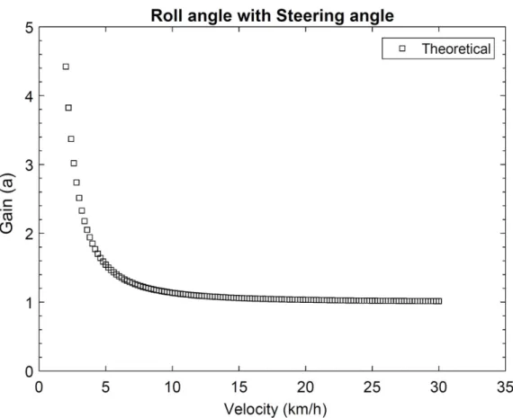
2.5 The theoretical gain for roll angle with steering angle . . . . 24

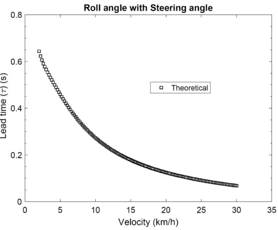
2.6 The theoretical delay time for roll angle with steering angle . . . . 25

2.7 Root-locus plot for open-loop motorcycle system. . . . . 26

2.8 Regions of stability for different values of roll angle gain a and lead time τ for closed-loop system of the motorcycle. . . . 27

3.1 Instrumented motorcycle for the experiments . . . . 29

3.2 Steering angle and roll angle curve of a rider normalized in [−1,1] range at 3.1 km/h. . . . 32

3.3 Validation of theoretical gain . . . . 35

3.4 Validation of theoretical delay time . . . . 35

3.5 Steering angle and steering torque correlation with roll angle . . . . 36

3.6 Validation of theoretical results from experiments for expert riders. . . . . 37

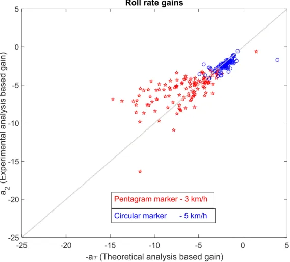
3.7 Validation of roll rate gain values based on theory and experiments. . . . 38

3.8 Riders BMI versus their age. . . . 40

3.9 Riders BMI versus their riding experience level. . . . 41

3.10 Validation of theoretical results from experiments for all riders. . . . 42

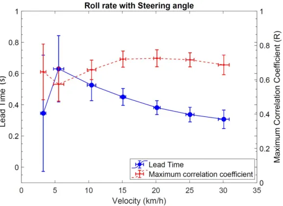
3.12 Maximum correlation (R) and lead time for roll rate with steering angle . . . . . 44

3.13 Maximum correlation (R) and lead time for yaw angle with steering angle . . . . 45

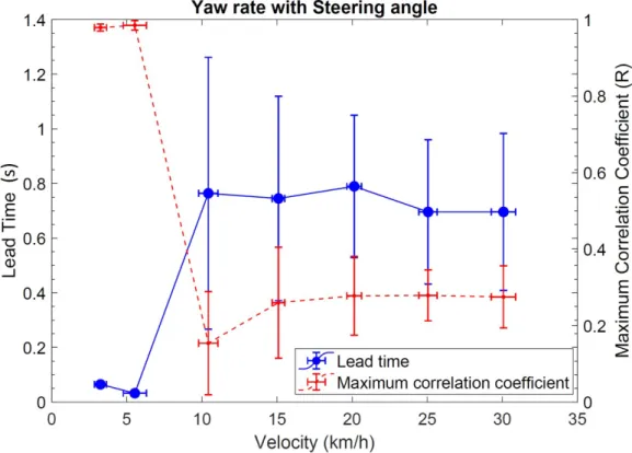
3.14 Maximum correlation (R) and lead time for yaw rate with steering angle . . . . 46

3.15 Maximum correlation(R) and lead time for roll angle with steering torque . . . . 47

3.16 Maximum correlation(R) and lead time for roll rate with steering torque . . . . 47

3.17 Maximum correlation(R) and lead time for yaw angle with steering torque . . . 48

3.18 Maximum correlation(R) and lead time for yaw rate with steering torque . . . . 49

3.19 Multiple correlation of roll angle and roll rate with steering angle and steering torque . . . . 50

3.20 Lead time and multiple correlation(R) for steering torque with steering angle . . 51

3.21 Multiple regression coefficients for roll angle and roll rate with steering angle . . 52

3.22 Multiple regression coefficients for roll angle and roll rate with steering angle . . 53

3.23 Steering angle prediction validation at 3.1 km/h . . . . 54

3.24 Steering angle prediction validation at 5.8 km/h . . . . 54

3.25 Gain values of the roll angle for various riders experience levels at different speeds. 55 3.26 Gain values of the roll rate for various riders experience levels at different speeds. 56 3.27 Regression correlations for various riders experience levels at different speeds. . . 56

4.1 Control algorithm to balance the motorcycle. . . . . 59

4.2 Stability Control of the motorcycle . . . . 60

4.3 Maximum correlation coefficient between the steering angle and the steering torque. 61 4.4 Values of the G

for estimating steering torque from steering angle . . . . 62

4.5 Lead time values for the steering torque with the steering angle. . . . 63

4.6 MBD Model of the motorcycle . . . . 64

4.7 Fast Fourier transform of the steering angle and the roll angle @ 3km/h. . . . . 66

4.8 Plant Export for ADAMS Control . . . . 67

4.9 Motorcycle speed during the co-simulation. . . . 69

4.10 Comparison of actual and estimated steering angle in simulation. . . . 70

4.11 The steering torque estimated from the analysis applied to the motorcycle model. 70

4.12 Roll angle result from the simulation. . . . 71

4.13 Yaw and roll rate results from the simulation. . . . 72

4.14 Directional control model for the motorcycle . . . . 73

4.15 Speed of the motorcycle while taking a turn . . . . 74

4.16 Steering torque and steering angle while taking a turn. . . . 75

4.17 Roll angle and yaw angle while taking a turn. . . . 75

4.18 Lateral displacement versus longitudinal displacement while taking a turn. . . . 76

4.19 Roll rate and yaw rate while taking a turn. . . . 76

A1 Spring and damper properties of the front and rear suspension systems of the

motorcycle . . . . 88

List of Tables

1.1 Number of automobile sales in India over the past few years [5]. . . . 2 2.1 Layout parameters of the motorcycle. . . . 17 2.2 Input and output parameters used in linear model. . . . . 18 2.3 Layout, mass and inertia of the motorcycle including a rider weighing 65 kg. . . 23 3.1 Details of the sensors used in experiments. . . . 30 3.2 Averages and standard deviations of motorcycle speed (v) and roll angle gain (a). 34 A1 Mass, center of gravity and inertia properties of various subsystems of the mo-

torcycle. The center of gravity and moment-of-inertia matrices are defined with respect to a maker on the vehicle in ISO coordinate systems. . . . . 89 A2 Front and rear tires properties of the motorcycle used in the MBD model. All

other coefficients such as longitudinal, lateral, overturning, scaling, rolling and

aligning are same between the tires. . . . 90

A3 Details of different riders selected for the experiments. . . . 94

Chapter 1

Introduction

1.1 Introduction

Motorcycles are a preferred mode of daily transportation in many countries. The reasons for their popularity are traffic congestion caused by increased population and underdeveloped road infrastructure; and because they are the most economically viable option. The increased traffic and poor road infrastructure constrain them at extremely low speeds. The motorcycles are unstable at these speeds and require continuous inputs from the riders to attain stability.

These inputs cause fatigue to them, and the low-speed instability is a safety concern for them.

Therefore, this research presents a study on the low-speed stability of motorcycles.

This chapter has been broadly divided into four sections. Firstly, the background section presents the reasons for the reduced speeds of motorcycles and related concerns to the riders.

This section shows that the increased traffic, poor economic condition and increased population

result in increased motorcycles sales and traffic congestion. These situations reduce the average

speeds of the motorcycles and their poor stability at low-speeds is physically tiring and a safety

concern for riders. Secondly, a review of past studies on motorcycle dynamics presents brief

details about their development from the stability point of view and parameters affecting it, in

the literature review section. The past studies show the limitations in improving the low-speed

Thirdly, the scope and motivation of the research has been derived from the problems discussed in the background section and gaps found from the literature review section. It is found that there is a demand for dedicated research in the area of low-speed stability from increasing customers and traffic congestion. Therefore, there is a scope of studying the dynamics of the motorcycle to improve the low-speed weave and capsize mode instability, using an additional steering control system. Finally, the last section of this chapter presents a brief overview of each chapter of this thesis.

1.2 Background

The population of the world has been increased every year, especially in developing countries, as shown by the population reference bureau (PRB) [1]. The increased population increased the number of vehicles such as car, buses, trucks and taxis on the road, every year in different countries [2, 3]. Table 1.1 shows that the numbers of automobiles have been increasing in India.

The number of motorcycles has increased from 14.8 million in 2013-14 to 21.1 million in 2018-19 [4, 5]. PRB also shows that the number of poor people earning less than $1.25 per day has been declined significantly over the years. It shows that their relative purchasing power has increased. These people are the main contributor to the increasing demand for the motorcycle as it is the most affordable motorized vehicle available.

Table 1.1: Number of automobile sales in India over the past few years [5].

The increased number of vehicles causes traffic congestion. The reasons for these situations are insufficient infrastructure and lack of a balanced traffic system, as shown by Mahmud et al. in their research on the cause and effect of traffic jams in Dhaka [6]. Similar traffic conditions exist in many cities and developing countries that constrains the speeds of motorcycles. It becomes challenging for novice riders to stabilize them at these speeds; therefore, these riders need a motorcycle with enhanced stability. There are many research studies on high-speed stability [7, 8, 9]. Whereas, limited research studies available focused on low-speed stability of the motorcycles, as discussed in the next section.

Figure 1.1: Root-locus plot for the stability of a motorcycle[10].

There are three major out-of-plane modes of the instability of motorcycles:

1. Capsize: it is a non-oscillating mode that is mainly controlled by the rider;

3. Wobble: it is an oscillation of the front steering system including front wheel about the steering axis which does not involve the rear frame in any significant way.

Figure 1.1 shows the root locus for the lateral modes, including above mentioned three out-of- plane modes. The arrows show the direction of an increase in speed for the modes. The weave and capsizes modes are unstable at low speeds, as shown in the figure; therefore, this research focuses on improving them.

Many motorcycle manufacturers such as Piaggio [11], Honda [12] and BMW [13] proposed the concept of a three-wheeled motorcycle. The third wheel takes support from the ground to improves the low-speed capsize and weave stability. Although they designed these concepts for the dynamics similar to that of a motorcycle, they can not match it, especially the steering control and roll behavior. These concepts also confirm the saturation in improving the low- speed stability of conventional motorcycles. Popov et al. [7] have reviewed the literature on the motorcycle’s control. It shows that limited research studies are available on low-speed stability.

And, there is a scope to study and improve it using electronic control systems. Furthermore, this system can be useful to reduce the human hazard involved in some future development tests.

1.3 Literature review

This section presents a review of the research studies on the stability of the motorcycles. It includes the historical development of single-track vehicles, such as bicycles and motorcycles from the stability point of view. The research studies show that some design variables are crucial for motorcycles stability; however, they have limitations to improve it at low-speeds.

The motorcycles are unstable at extremely low-speeds; but, additional inputs from rider can

stabilize them [14]. Therefore, many authors presented advanced devices and methods, that in-

crease low-speed stability such as steering actuator systems, gyroscopic moments and additional

balancers.

Riders inputs are crucial for the motorcycles performances, which are from steering, body movements, thighs etc. They change with motorcycles speeds, types of maneuvers and rider experience levels; therefore, investigating them are also important for motorcycle stability. The effects of rider experience levels on the low-speeds stability of a motorcycle are discussed in this section to find the suitable rider model.

1.3.1 History of single-track vehicles

The evolutionary development of single-track vehicles took place during the 19

century.

The first commercially successful two-wheeled, steerable and human-propelled machine was

“Draisine walking machine,” commonly called a “Velocipede,” developed by German Baron Karl Drais in 1818. The development from the Draisine walking machine to the more stable

“Safety bicycle” was the most important in the history of the bicycle [15]. John Kemp Starley developed the safety bicycle in 1885. It featured a steering system including front wheel, equally sized wheels and a chain drive to the rear wheel. It changed the perception of the single-track vehicles from a dangerous one to a daily mode of transportation for people. All the motorcycles of today have a similar layout as that of the safety bicycle. It shows that the domain of research for the layout and mass distribution optimization has been saturated for any significant gain in motorcycle stability. Although, minor improvements on them to improve maneuverability, riders efforts, speeds of the motorcycles etc. have been done.

Whipple was first to develop the theoretical model for a single-track vehicle to predict the

instability modes [16]. This model has been a benchmark model and experimentally validated

by many researchers. Sharp was first to develop the theoretical model for motorcycle stability,

that includes a proper tire model [17]. Eaton [18] has validated this model experimentally

on a motorcycle using the Weir’s rider model [19]. Similarly, many authors investigated and

presented a theoretical model for single-track vehicles.

1.3.2 Motorcycle stability

Motorcycles are unstable below the certain critical speed [17, 20]. Moreover, the required steering input or the gain value for the stability increases as speeds reduce [21]. Therefore, it is challenging to balance a motorcycle at low-speeds, especially for new riders. They become very cautious as it requires continuous input from them at such speeds [22]. It causes fatigue and a safety concern for them. Therefore, in this research, the focus is to improve the low-speed stability of the motorcycles.

The stability of a motorcycle is a function of its geometry and mass distribution. Cossalter has performed detailed studies on parameters such as caster angle, wheelbase, trail and mass- distribution for their effect on motorcycle stability [10]. The results of these studies determined the directional change in them. For example, changing the trail value from positive to negative makes a rideable bike un-rideable [23]. Doyle has conducted experiments on a bike, with zero trail values, zero caster angle and zero mass offset in the front steering system [24]. He found that it eliminates the roll angle of a bicycle to steer coupling; thus, no effect of steering input by the rider in such vehicles. In general, the center of gravity of a motorcycle lies longitudinally between the ground contact points of both front and rear wheels. The significant change in it towards the front of the ground contact point of the front wheel can stabilize a two-mass single-track vehicle having a negative trail [25]. It shows that the layout and mass inertia are inter-dependent for stability. However, the feasibility of such modifications is debatable.

The layout and mass distribution of the motorcycles can not be entirely modified for sta-

bility. They also influence other performance requirements, such as maneuverability, com-

fort, ergonomics, acceleration feel and braking. Although, all these changes can not self-

stabilize the motorcycle at extremely low speeds below 7 km/h [25]. Therefore, it becomes

necessary to explore other methods of improving them. Many research papers are available

those discusses high-speed stability (weave and wobble) and handling characteristics of motor-

cycles [26, 27, 28] . Whereas, limited studies available on low-speed stability, those evaluate

the rider inputs [7, 29, 30]. Therefore, it is the scope of the present research.

Motorcycles require precise control inputs from their riders for balancing below the critical speeds [20]. They balance it at low-speeds, even at 3 km/h [14], which shows that they provide additional stability to the motorcycles at low-speeds. Therefore, it is necessary to model an appropriate rider model for developing a system that can stabilize them at low-speeds. The riders models presented in the past are discussed next in this section.

1.3.3 Motorcycle rider modeling

The rider models can be developed specifically to the riding or test conditions. Many research studies show that the riders use different body inputs during different maneuvers such as steering input while riding on a straight path and their lean torque during cornering to achieve precise control of motorcycles. Some rider models for motorcycle control are as follows: a rigid body rider that is rigidly connected to the main rear frame for motorcycle stability [16]; two-piece body such that the lower part rigidly attached to the rear frame and the upper part behaves like an inverted pendulum on rear frame, with stiffness provided by spring and damper for bicycle stability and control [20]; upper body can steer, lean and move laterally; and more realistic multi-body riders, including full muscle-skeleton models for assessing the riders, accurately [31].

The present research also requires an accurate rider model. Therefore, this section presents the relevant studies that comment on rider actions at low-speeds.

Doria et al. [32] determined the degree of freedom required for a rider model that achieves

similar motion and torque frequency responses to that during the experiments. They used a

simulator that provided different frequency inputs to the bicycle mockup. The results showed

that the phase of the rider motion response at low-frequency input was close to zero. Whereas,

the roll displacements of the rider trunk was higher than that of a bicycle. Therefore, the

rider can be a rigidly mounted with the frame, and the higher gain for the rider lean can be

compensated in the vehicle roll angle gain. Kooijman et al. [33, 34, 35] conducted experiments

on a large treadmill using an instrumented bicycle. The results showed that a very little rider

upper-body lean occurs while balancing them. Whereas, it is achieved mainly by steering

various speeds who adjusted to riding on treadmills. Cain et al. [36] show that the skilled and novice riders exhibit similar balancing performance using their lean at the low speeds. These research studies showed that the rider lean does not contribute significantly to the low-speed stability of bicycles. Moreover, the mass of motorcycles is much higher than that of bicycles;

therefore, the influence of riders’ lean on them will further reduce. It shows that a rigidly attached rider to the motorcycle frame can stabilize it through steering torque control.

Riders control motorcycles differently based on their experience. Prem et al. [37] found that the skilled rider provides a larger steering angle and have a shorter reaction time than a novice rider for a successful maneuver. Also, the novice riders showed more inter-rider variability than the experienced riders. Rice and Kunkel [38] and Prem and Good [37] found that the time-lag in the input is more important than its amplitude. They compared the magnitude of the steer or lean control for successful and unsuccessful runs for the same rider, during lane change experiments with both experienced and novice riders. Thus, this research presents the influence of different riders experiences on motorcycle control at low-speeds. The variations in gain values and response time were observed with their riding experience.

controllers for motorcycles: The past research studies divide the controllers used for mo-

torcycles broadly into two categories: classic and modern control. In classical control approach,

the system identification method is used to determine the gain values that includes time delays

between input and output signals. In optimal control, the strategy is to minimize the cost

function of the state or control variables using state-space techniques to achieve optimum per-

formance [39]. Schwab et al. [33] found that the roll feedback gains become unrealistically

large at low speeds for roll stability using the optimum controller (LQR). They found that

the system has marginal stability and requires more realistic steer torque feedback gains for

determining the feedback gains. The cost function optimization does not relate directly to

the human-like controller. Hence, optimal control is unsuitable for developing a controller for

the rider’s feel. Also, there are some other control strategies for motorcycle control such as

fuzzy logic, neural network, forward dynamics and inverse dynamics controllers. Although, the

classic control strategies are better for studying rider actions, and developing controllers based

on that. Popov et al. [7] reviewed the modeling of the control of motorcycles. It showed that the classical control method is promising for determining the gain values based on actual rider control behavior. Therefore, the present research opted classic control approach for developing a controller for low-speed stability.

1.3.4 Improved stability from additional systems

Adding new systems to the motorcycles can improve their stability, especially at stationary and low-speeds. These systems include additional steering systems, gyroscopic systems and other balancing systems. This section presents brief about these systems.

Additional steering systems: In past research studies, the authors used two kinds of steering

inputs for controllers: steering angle and steering torque. Weir [19] found that the rider uses

steering torque associated with the rider lean to stabilize the motorcycles. He applies this

input determined from the state parameters of the vehicle. The results of the study show

that the amplitude of the rider input depends on the motorcycle state. It also has some delay

due to human limitations. Eaton [18] used steering torque to investigate the stabilization

of the motorcycle roll angle. He restricted the rider’s body motion by a rigid brace during

the experiments. However, there was a significant difference in his model from experimental

results for speeds below 40 mph. In research studies on motorcycle maneuverability at medium

speeds, [40, 41] found that the inputs to the motorcycle are mainly from the steering, more

specifically steering torque. And, other rider inputs do not contribute to the motorcycle control

and probably there for the rider’s comfort. Rice [42] measured both the steering torque and

steering angle with outputs such as rider lean, roll angle, yaw rate and lateral acceleration for

motorcycles. Ruijs et al. [43] used steer torque control based on a Sharp [17] motorcycle model

with tires and leaning rider to identify the controller gains for stability at speeds from 5 m/s

to 60 m/s. However, in the above-mentioned research studies, the target speeds were relatively

higher.

Many authors presented the concept of autonomous single-track vehicles based on added steer- ing systems. A small humanoid robot can balance and steer a scaled-down bicycle by providing input to the handlebar using the lateral dynamics [44]. A mathematical model of the bicycle and motor with a controlled algorithm can reduce the effort of applying the steering angle for balancing it [45]. Tanaka et al. used steering control for balancing their bicycle robot, using the dynamic model derived from the equilibrium of gravity and centrifugal force [46]. Lenkeit [47] developed a motorcycle robot using steer angle control at a low speed below 30 km/h, and steer torque control at high speed above 30 km/h for path control. The results showed that the robot control was good at speeds below 20 km/h and above 35 km/h; whereas, it had low damped oscillations between these speeds. Many other authors examined the relations between input and output parameters of a motorcycle to construct a rider robot [48, 49, 50, 51, 52]. In these research studies, the target speeds were relatively higher. Also, these robots balanced the single-track vehicles using the controller input determined without assessing the actual rider inputs. Whereas, in the present research, the low-speed stability of the motorcycle is studied using an experimental approach with many riders.

Gyroscopic systems: Gyroscopic systems discussed in past studies provided two types of

control using gyroscopic moments to balance the single-track vehicles: either the gyroscopic

precession or the adjustment of the gyro speed [53, 54, 55]. These moments supported the

single-track vehicles at low-speeds. Benzos et al. [53] used two identical gyroscopic rotors

located between the bicycle wheels, sealed with the frame to pivot relative to the chassis. The

pivot axis was perpendicular to the vehicle-plane of the bicycle. They assembled the rotors

with a gear train to turn them by the same angle and speeds in the opposite direction. These

ensured their vectors of kinetic momentum in opposite directions, which generated gyroscopic

moments to balance the bicycle for any disturbance in the roll direction. Lot et al. [54] proposed

that the most effective configuration for gyroscopic rotors are when they spin with respect to

an axis parallel to the wheels’ spin axis and swing with respect to the vehicle yaw axis. They

also showed that the actively controlled gyroscopes are capable of stabilizing the vehicle in its

whole range of operating speeds with negligible change in handling characteristics. Karnopp

[55] showed a relatively simple tilt control system using a gyroscope. This system was capable of stabilizing the vehicle at stationary, or on a low traction surface. Furthermore, the system could achieve a coordinated turn on high traction surfaces. However, the cost for this system was high; hence, it is questionable, whether they are reasonable. These systems also deteriorate the dynamics of the motorcycles by slowing them down. These systems do not provide balancing inputs similar to that of a rider, as the system behavior coupled with the steering input by them was not studied. Therefore, usage of such stability enhancement tool is questionable.

Other balancing systems: In research [56], the motorcycle achieved the low-speed stability by steering provided to both front and rear wheels, different from their typical design. However, these changes may not retain the conventional form and dynamics of the motorcycle. Yi et al. [57] designed a nonlinear controller to handle the vehicle balancing. The motorcycle balancing is guaranteed by the system internal equilibrium calculation and by the trajectory and system dynamics requirements. Kimura et al. [58] reduced the steering input required to improve the low-speed stability of motorcycles by adding an extra degree of freedom to them using a mechanism.

There are several other methods have been attempted to improve the stability of single-track vehicles at low-speeds using balancer systems. Keo et al. [59, 60] proposed a double inver- ted pendulum (roll and lean angle) stabilization model for the bicycle. They found that the stabilizing it using gyroscopic flywheel performed better than a balancer [59]. Whereas, the gyroscopic systems cannot control the roll angle to the desired value, unlike the balancer. Since the flywheel and the balancer have different advantages for stabilizing the bicycle, they used both; and validated using experiments. In another similar research, Keo et al. [60] presented a control strategy of an autonomous electric bicycle with both a steering handlebar and balancer.

They showed that a steering handlebar and a balancer had better performance for balancing

than with only a balancer using simulations studies. The balancer system worked under unex-

pected disturbances for stabilizing the bicycle but worked only at low speed. It behaved like a

double pendulum due to its ability to steer at high speeds. However, stabilization and tracking

mass control. Also, an inverted pendulum or laterally moving mass required higher gains than the steering control.

In summary, the past research studies showed that the improvements in low-speed stability in a conventional way by tuning the parameters such as layout and mass distribution has no significant improvements. Thus, the authors investigated other methods for improving it using controllers. They attempted rider models for motorcycle dynamics; however, their focus has been on tracking control (directional control) and stability control at higher speeds. Few of them developed new support systems such as gyroscopic, steering and balancer systems, to balance single-track vehicles at low-speeds. However, their approach was to attain the balancing from control engineering requirements. It showed that extensive study using different riders had not been performed to develop a controller that balance the motorcycles similar to the riders. Therefore, a gap is found to construct steering support systems using experimental study with different riders that improve the motorcycle’s stability at extremely low-speeds (≤

5 km/h).

1.4 Scope and motivation of the thesis

The population, poor infrastructures and financial condition of people in many countries have increased the demand for motorcycles. Therefore, they become the most popular mode of transportation there in many countries. These situations cause traffic congestion and restrain them at low speeds. They have poor stability at these speeds and require active input from the riders. It causes fatigue to them, and it is a safety concern. These issues motivated us to do dedicated research to improve the low-speed stability of motorcycles.

The scope of the research has derived from the gaps identified in the literature review section. It is found that there is a scope of developing a steering support system by experiments with dif- ferent riders that improve the stability of the motorcycle at extremely low speeds (≤ 5 km/h).

Therefore, a theoretical, experimental and simulation methods have been presented in this

research to develop and validate the same. The theory defined the stability regions for a mo-

torcycle, which were validated by the preliminary experiments with expert riders. It provided

conviction for performing an extensive experimental study. Then, detailed experiments with

riders from various experience levels were conducted. The experimental results were analyzed

using statistical methods to identify critical parameters for stability. These parameters were

used to determine the gain values for a control algorithm to estimate the steering input to

balance the motorcycle. The control algorithm was developed based on this steering estima-

tion and modeled in Simulink. The Simulink control model was co-simulated with a validated

motorcycle model in MBD software, VI-Motorcycle. In general, the default controller of the

software can not balance any motorcycle model at speeds below 10 km/h. Whereas, the simu-

lation results verified that the software could balance the MBD model at extremely low speeds

using the control algorithm developed in this work.

1.5 Overview of each chapter

This thesis is broadly divided into three stages. Firstly, a theoretical model for the stability of the motorcycle is presented that determines the low-speed stability regions. These regions showed gain values required for the steering input and delay in it, with respect to the motor- cycle state required for stability. Secondly, experiments have been performed that validated the theoretical model and identified the input and output parameters of the motorcycle critical for balancing it. A control algorithm developed based on these parameters is modeled in Sim- ulink. It is integrated with a validated MBD model of the motorcycle prepared in commercially available software, VI-Motorcycle to perform simulation studies. These stages are described in the following chapters:

Chapter 2 presents a mathematical model for the low-speed stability of the motorcycle. It determines the stability regions that show the roll angle gains and corresponding lead time to stabilize them at low-speeds.

Chapter 3 presents the experiments details and method of analyzing them. At first, preliminary experiments with expert riders validated the theoretical results from Chapter 2 that provided assurance for further study. Then, detail experiments with riders from various experience levels were performed to identify critical parameters for low-speed stability. The chapter also presents a control algorithm based on these parameters.

Chapter 4 presents the co-simulation studies between the control algorithm modeled in Simulink and an MBD model of the motorcycle in VI-Motorcycle. The simulation results show that the control algorithm can balance the motorcycle model successfully.

Finally, Chapter 5 presents the conclusions and future scope of the research.

Chapter 2

Theoretical Model for Stability of a Motorcycle

2.1 Introduction

Various internal and external forces are applied to motorcycles when in motion, which influences

their stability. This section presents a linear mathematical model for their low-speed stability

using these forces. The model determines characteristic equations for the motorcycle stability in

the roll direction for open and closed-loop systems. Stability regions for the motorcycle stability

have determined from these equations. A motorcycle rider must apply steering inputs inside

these regions to balance them. In this research, a scooter-type motorcycle has been selected

for studying the low-speed stability. The brief details of the motorcycle layout, specifications

and mass-distribution are provided in this chapter. The results of the theoretical analysis for

the motorcycle are also discussed in this chapter.

2.2 Linear model for motorcycles

Figure 2.1 shows the schematic of a motorcycle and a rider system to achieve the low-speed stability. It shows that the rider estimates the required input to balance it using their state as feedback. The objective of the rider is to stabilize it by maintaining the reference values of the state parameters (i.e., roll rate φ ˙ = 0 and roll angle φ ≈ 0 in this case). The reference value for the roll rate is zero to achieve steady-state condition. Ideally, the reference values for the roll angle should also be zero for symmetric motorcycle moving in a straight path. Although, it can have a small offset due to the lateral center of gravity of motorcycles and while they take a turn.

The disturbances presented in the model are due to the rider disruptions and road irregularities.

These disturbances are a component of the input and the output parameters of the motorcycle respectively. The disturbances by the riders become an input to the motorcycle and influences the output parameters. Similarly, the road disturbance on the motorcycle changes the output parameters that influence the rider input. This relationship between the input and output parameters are studied to achieve the low-speed stability, as shown in the next section.

Figure 2.1: Block diagram for the low-speed stability of a motorcycle and rider system.

Figure 2.2 shows the schematic of a typical motorcycle. It shows the layout and mass-inertia

parameters important for motorcycle stability. These parameters are listed in Table 2.1.

Table 2.1: Layout parameters of the motorcycle.

Parameters Symbols

Fork offset d

Wheelbase l

Castor angle

Radius of the front wheel r

Radius of the rear wheel r

Front wheel contact point with the ground A

Rear wheel contact point with the ground O

Point where the projection of steering axis intersects with the ground B Longitudinal center of gravity of the rider-motorcycle system from point O l

Vertical center of gravity of the rider and motorcycle system from point O h Mass of the steering system including front wheel assembly M

Front steering system inertia including wheel about the steering axis I

Height of the center of gravity of the steering system from the ground h

Roll inertia of the rider and motorcycle system about its center of gravity I

Shortest distance between center of gravity of front steering system (including d front wheel assembly) and steering axis

Roll axis of the motorcycle x-axis

Figure 2.2: A typical layout of a motorcycle.

Table 2.2: Input and output parameters used in linear model.

Parameters Symbols

Speed v

Roll angle φ

Yaw angle ψ

Steering angle δ

Kinematic steering angle δ

Lateral displacement at O y

Instantaneous turning circle radius R

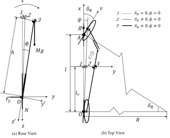
Figure 2.3: Schematic of linear model of motorcycle showing its different states.

Schematic Figure 2.3 depicts different states of the motorcycle while balancing. The symbols

used in the figure are listed in Table 2.2. The figure shows that a motorcycle-rider system (mass

M ) at first steered by an angle (δ) and then rotated about roll axis (x -axis) by an angle (φ), as

shown by Legend 2 and Legend 3, respectively. These angles are generated due to disturbances

to the system and input by riders to balance it. Figures 2.3a and 2.3b show rear-view and

top-view of the system respectively. Various forces acting on the motorcycle are due to weight

(M g), normal reaction (N ) and lateral force (F

) as shown in Figure 2.3a. Figure 2.3b shows the effect of steering angle (δ) and roll angle (φ) on the motorcycle state. Marginal changes in δ and φ result in yaw angle (ψ), which makes the motorcycle to follow a circle of radius R.

The significance of the steering mechanism on the stability of the motorcycle is described in this section.

Equation of motion

The equation of motion for the stability of the motorcycle in roll direction about the x -axis (the axis intersecting vehicle plane and ground plane at point O) is as follows:

I

φ ¨ + M y ¨

h = M ghφ + M

+ M

+ M

, (2.1)

where:

I

is the roll inertia of the motorcycle with respect to point O, which is defined in terms of roll inertia about center of gravity I

as follows:

I

= I

+ M h

. (2.2)

The lateral acceleration of the motorcycle y ¨ about point O is a function of the centrifugal acceleration a

and lateral velocity v

as follows:

¨

y

= f (a

) + f (v

)

These functions can be defined in terms of the forward velocity v and kinematic steering angle δ

as follows:

¨

y

= f (v, δ

) + f (v, δ ˙

)

¨ y

= v

l δ

+ v l

l

δ ˙

. (2.3)

Gyroscopic moments on the motorcycle is a function of rotations of both front and rear wheels (ω

and ω

respectively). Additionally, it also depends on the steering rate δ ˙

as follows:

M

= f (ω

, ω

, δ

) + f ( δ ˙

)

M

= − v

l

I

r

+ I

r

δ

− v

r

I

δ ˙

(2.4)

Moment due to the front steering system vibration is defined as a function of steering acceler- ation δ ¨ as follows:

M

= f ( δ) = ¨ −(I

+ M

dh

) δ. ¨ (2.5)

Moment due to the front wheel normal reaction force is defined as a function of steering angle δ as follows:

M

= f(δ) = M g l

l d

δ. (2.6)

The following equation is obtained by substituting the values from Equations (2.2)–(2.6) in Equation (2.1).

(I

+ M h

) φ ¨ + M

l

δ

+ v

δ ˙

h = M ghφ −

f w

rf

+

r

δ

−

f

I

δ ˙

− (I

+M

dh

) δ ¨ + M g

d

δ.

(2.7)

Further, the kinematic steering angle can be defined by the equation as follow:

δ

= tan

cos() sin(δ)

cos(φ) cos(δ) − sin(φ) sin() sin(δ )

. (2.8)

Equation (2.8) can be approximated in linear form for δ and φ → 0 as follows:

δ

≈ δ cos(). (2.9)

Substituting the value of kinematic steering angle from Equation (2.9) in Equation (2.7) gives the following equation:

(I

+ M h

) φ ¨ − M ghφ =

−M

v²

l

δ + v

δ ˙

cos()h −

f w

rf

+

r

cos()δ −

f

I

cos() δ ˙ − (I

+M

dh

) δ ¨ + M g

d

δ.

(2.10) The open-loop transfer function for the low-speed stability of the motorcycle system can be defined from Equation (2.10) by the following expression:

G

(s) = φ(s) δ(s) =

−M

v²

l

+ v

s

cos()h −

f w

rf

+

r

cos() −

f

I

cos()s − (I

+M

dh

)s

+ M g

d

(I

+ M h

)s

− M gh .

(2.11) The transfer function defines the stability of the motorcycle at all the speeds. The poles of the open loop systems are as follows:

s = ±

s M gh

I

+ M h

(2.12)

where,

M gh

I

+ M h

> 0

Equation (2.12) shows that one of the open-loop poles of the system is always positive. There- fore, the system is unstable, and its low-speed stability cannot be achieved. It requires a control input to attain low speeds stability making the system a closed-loop system. This mathematical model presents the closed-loop system for the motorcycle, using the roll angle as the feedback parameter and steering angle as the control input to attain the stability.

The closed-loop feedback of the motorcycle can be defined using the following relationship

between the steering angle (δ) and the roll angle (φ):

where a is gain value and τ is lead time for the roll angle with respect to the steering angle.

Equation (2.13) can be further simplified for τ < 1 as follows:

δ = a.φ − aτ φ. ˙ (2.14)

By substituting the value from Equation (2.14) in the Equation (2.10) following equation is obtained:

C

...

φ + C

φ ¨ + C

φ ˙ + C

φ = 0, (2.15) where,

C

= −(I

+ M

h

)daτ (2.16)

C

= M h

− M hl

v cos()aτ

l + I

+ (I

+ M

h

)da − I

v cos()aτ r

(2.17)

C

= M hv cos()a l

l − vτ l

+ I

v cos()a

r

− v

cos()aτ l

I

r

+ I

r

+ M gl

d

aτ

l (2.18) C

= v

cos()a

l

I

w

r

+ I

w r

− M gh − M a

gdl

+ hv

cos() l

. (2.19)

Equations (2.16)–(2.19) show constants C

, C

, C

and C

of closed-loop characteristic Equa-

tion (2.15). A motorcycle is stable when all the real-parts of Eigenvalues of the characteristic

equation are negative, for different values of the roll angle gain a and it’s lead time τ . The

next section presents the stable zones for the motorcycle used for experiments. It also shows

the results for their open and closed-loop stability.

2.3 Motorcycle specifications and theoretical results

2.3.1 Motorcycle specifications

The motorcycle chosen for the experiments is a small engine capacity scooter-type motorcycle.

Table 2.3 provides its layout, mass and inertia. The same table also shows the symbols corres- ponding to the parameters used in this thesis.

Table 2.3: Layout, mass and inertia of the motorcycle including a rider weighing 65 kg.

Parameters Symbols Values Unit

Total mass M 165.70 kg

Wheelbase l 1.236 m

Roll inertia at center of gravity I

18.79 kgm

Height of center of gravity from ground h 0.545 m Horizontal distance of CG from rear axle l

0.450 m

Caster angle 25.8 degree

Fork offset d

0.004 m

Front steering system mass M

17.72 kg

Front steering system inertia I

23.72 kgm

Height of front steering system CG from ground h

0.540 m Shortest distance: steering system CG and steering axis d 0.005 m

Front wheel rolling radius r

0.214 m

Front wheel spin inertia I

0.122 kgm

Rear wheel rolling radius r

0.205 m

Rear wheel spin inertia I

0.112 kgm

Acceleration of gravity g 9.81 m/s

Front suspension Rear suspension

Steering column

Frame

Front wheel

Rear wheel Engine

Steering joint

Engine-frame joint

Figure 2.4 shows a skeleton of the scooter-type motorcycle. It depicts various subsystem of the motorcycle.

2.3.2 Theoretical results

The values of the variables from the Table 2.3 are substituted in Equations (2.17–2.19). The motorcycle is stable when all these coefficients are positive as per Routh-Hurwitz stability criteria. The results of a and τ for the positive coefficients of characteristic equation for the speeds range of 3 to 30 km/h are shown in Figures 2.5 and 2.6, respectively.

Figure 2.5 shows that the roll angle gain a is constant above 10 km/h; whereas, it increases sharply below 10 km/h. Figure2.6 shows that the lead time gradually increases as speed reduces, and it is always positive.

Figure 2.5: The theoretical gain for roll angle with steering angle

Figure 2.6: The theoretical delay time for roll angle with steering angle

Further, the poles of the open and closed-loop system are shown in this section. Root-locus plot for the open-loop system Equation (2.11) shows that one of the poles of the system is always positive at speeds 3, 5 and 10 km/h, as shown in Figure 2.7. Therefore, the low-speed stability for the open-loop system of the motorcycle cannot be achieved.

The closed-loop system discussed in the above section determines regions for the motorcycle stability at low-speeds. The motorcycle is stable for the values of a and τ , where all the real parts of the eigenvalues are negative. There were three eigenvalues of the closed-loop characteristic equation: λ

, λ

and λ

. The stability zones of the motorcycle were defined from the following criteria:

Stable zone: Re[λ

] < 0 & Re[λ

] < 0 & Re[λ

] < 0.

Unstable zone: Re[λ

] > 0 or Re[λ

] > 0 or Re[λ

] > 0.

Figure 2.7: Root-locus plot for open-loop motorcycle system.

The shaded zones in Figures 2.8a and 2.8b show regions for the stable motorcycle corresponding

to the roll angle gain a and roll angle lead time τ at speeds 3 and 5 km/h, respectively. The

rider must be operating inside the shaded zone shown in Figure 2.8 to achieve the low-speed

stability. In the next chapter, the theoretical results have been validated from the preliminary

experiments results to get confidence for the detailed experimental study.

-25 -20 -15 -10 -5 0 5 10 15 20 25 -1

-0.8 -0.6 -0.4 -0.2 0 0.2 0.4 0.6 0.8 1

Roll angle gain (a)

Roll angle lead time ( (s))

Stable zone

(a) At 3 km/h.

-25 -20 -15 -10 -5 0 5 10 15 20 25

-1 -0.8 -0.6 -0.4 -0.2 0 0.2 0.4 0.6 0.8 1

Roll angle gain (a)

Roll angle lead time ( (s))

Stable zone

(b) At 5 km/h.

Chapter 3

Experimental Details, Analysis and Results

3.1 Introduction

In this section, the stability of the motorcycle detailed in the previous chapter has been studied

adopting an experimental approach. It was mounted with various sensors to measure the

required dynamic parameters. First, preliminary experiments with three expert riders were

conducted to validate the theoretical results at speeds 3 and 5 km/h. It also ensured that the

method of analysis of the experimental data provides useful results, and provided certainty for

further study. Next, detailed experiments with 19 more riders have been conducted for speeds

ranging from 3 to 30 km/h. The wide speed range was chosen to observe its influence on the

relationship between various input and output parameters of the motorcycle measured during

the experiments. The same method of analysis has been performed for both the preliminary and

detailed experiments. Different riders from a diverse background were participated to capture

the maximum possible variations in the results. A statistical method has been used to analyze

the experimental data to identify useful inputs and outputs parameters. An input estimation

model was formulated from regression analysis using these parameters and validated. It was

used for a controller for estimating input required for stability. This chapter presents, the

experiments, method of analyze them and results in detail.

3.2 Experimental preparations and methodology

3.2.1 Motorcycle instrumentation

The motorcycle shown in Figure 3.1 has been used for the experiments. Its specifications were given in Chapter 2. It was instrumented with two analogue sensors namely a potentiometer (range of linearity ±50

) and a piezoelectric sensor (range ±200 Nm and sensitivity −175 pC/Nm); an inertia measurement unit (IMU) (angular rate range ±400

/s with an angle meas- urement accuracy of 0.2

); a GPS antenna; and a data-logger which has a sample rate of 100 Hz . The brief details of the sensors mentioned above are shown in Table 3.1.

Figure 3.1: Instrumented motorcycle for the experiments

The torque sensor and potentiometer were connected to the data-logger using a de-connector

to the analog port. The INS was connected to the data-logger using a serial cable. The

GPS antenna was connected to the INS, which measures the speed, position and state of the

motorcycle. These sensors were first calibrated for their accurate values and then used for

Table 3.1: Details of the sensors used in experiments.

Sensors Descriptions

Torque Sensor

The sensor used to measure the steering torque was from KISTLER that can measure up to ± 200 Nm about an axis perpendicular to flanges used to mount it [62]. It was a Quartz sensor for measuring quasi-static or dynamic torque acting around its axis. It had several shear-sensitive quartz plates inside, which is kept between the two steel disks. Quartz exhibits the piezoelectric effect. The strain given onto the crystal produces an electro-motive torque which was a measure of steering torque.

Potentiometer

The potentiometer (sometimes called a pot) was used to measure the steering angle in terms of the voltage difference. It was from 2D [63]. In a linear potentiometer, change in angle result in a linear change in voltage.

A variable resistor inside it changes the resultant resistance of the potentiometer with the angle of rotation. Hence for the same current supply, the voltage changes and gave a measure of the change in the angle.

Inertia Navigation System (INS)

The INS system used for measurement of the roll, pitch and yaw angles and its corresponding velocities was Ellipse2-N from SBG system. It was a small-sized high-performance sensor with integrated L1 global navigation satellite system (GNSS) receiver [64]. It had low noise gyroscopes and efficient vibrations handling. Its accuracy was 0.1

for roll

and pitch angles and 0.5

for heading.

Global Positioning System (GPS)

Antenna

A magnetic patch antenna was used to obtain vehicle velocity and &

position through GPS tracking. It was directly connected to the INS sensor to measure velocity. The antenna used for the experiments was RLACS156 from VBOX [65].

Data-logger

Above mentioned sensors were connected to a data-logger known as VBOX 3i [66]. It used a powerful GPS/GLONASS receiver logging data 100 times a second (100 Hz) to achieve high-level accuracy.

These sensors were mounted on the motorcycle for the experiments. The rotating shaft of the

potentiometer was mounted on top of the handlebar, and its non-rotating body was fixed to the

frame. The handlebar and front steering system were disassembled to mount the piezoelectric

sensor. Two flanges were fixed to them such that the faces of the flanges were perpendicular to

the steering axis. The sensor was mounted between these flanges under high preload. The IMU

was mounted on top of the pillion seat, and the GPS antenna was kept on a metal plate fixed

to the rear frame of the motorcycle at the highest point on the motorcycle. The experiments

were conducted using this instrumented motorcycle.

3.2.2 Experimental details and method of analysis

Experimental procedures

Experiments were conducted on a proving ground using the motorcycle instrumented with aforementioned sensors at speeds 3 – 30 km/h. The motorcycle was ridden on the same dry asphalt road to inhibit the road variations in the results. The riders were instructed to follow a straight line marked on the proving ground, and not keep their foot down in order not to take any support from the ground. The experiments were conducted mainly to focus on balancing the motorcycle. Twenty-two riders those belong to a different age, gender, height, weight and experience, participated in the experiments as shown in Appendix-5. Different riders are chosen to capture the maximum variations possible in the results.

Method of analysis

The experimental data were divided into the sample size of 300 (i.e., 3 s) to examine the

instantaneous input and output parameters while balancing the motorcycle at low speeds. The

maximum correlation coefficient (MCC) and the lead time between these parameters were

calculated. Steering angle and steering torque were selected as the input parameters; roll and

yaw angles and their corresponding velocities were selected as the output parameters for the

analysis. The MCC defined herein as a cost function to determine the maximum possible

correlation between the input and the output parameters by shifting the output parameter

over the input parameter. The time step at which the cost function became maximum was

defined as the lead time. The MCC is a measure of the dependency of the input parameter on

the output parameter, and the lead time indicates the usability of the output parameter by the

rider for predicting the steering control.