Extension of Comparative Analysis of Estimation Methods for Dirichlet Distribution Parameters Halid M.A. and Akomolafe A.A.
*Department of Statistics, Federal University of Technology, Akure, Nigeria
* [email protected]
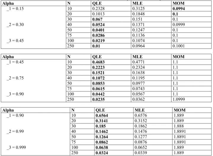
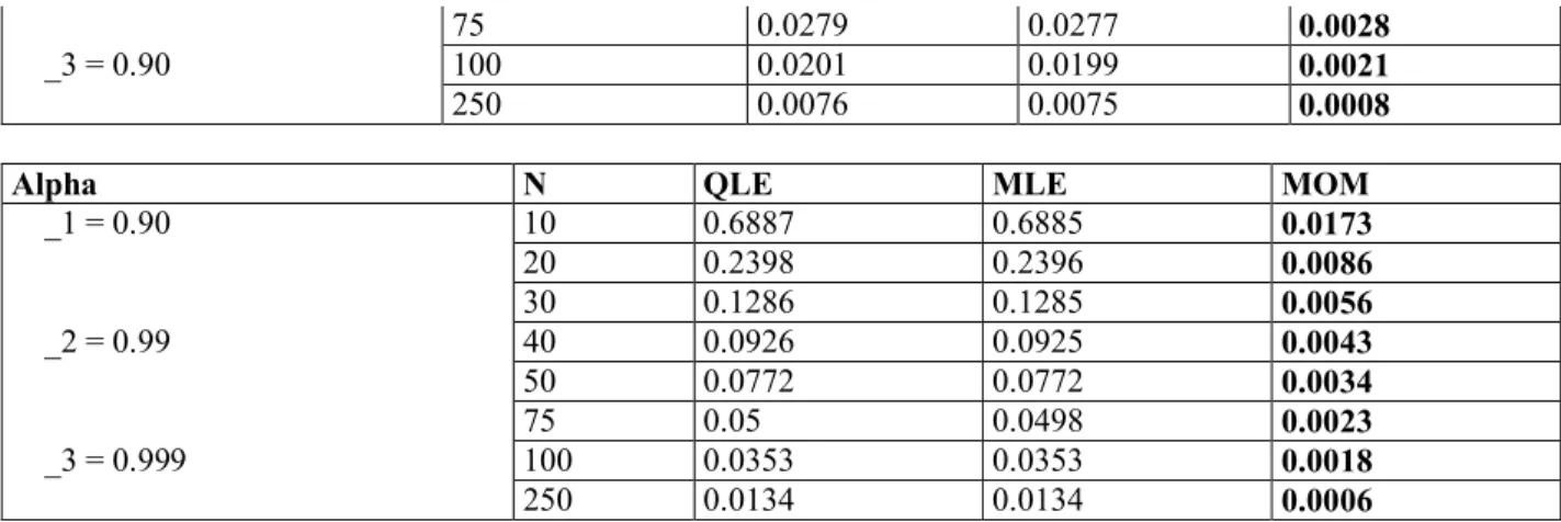
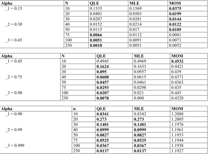
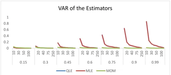
Abstract: The Dirichlet distribution is a generalization of the Beta distribution. This research deals with the estimation of scale parameter for Dirichlet distribution with known shapes. We examined three methods to estimate the parameters of Dirichlet distribution which are Maximum Likelihood Estimator, Method of Moment Estimator and Quasi- Likelihood Estimator. The performance of these methods were compared at different sample sizes using Bias, Mean Square Error, Mean Absolute Error and Variance criteria, an extensive simulation study was carried out on the basis of the selected criterion using statistical software packages as well as the application of the criterion to real life data, all these were done to obtain the most efficient method. The simulation study and analysis revealed that Quasi- Likelihood Estimator perform better in terms of bias while Method of Moment Estimator is better than the other two methods in terms of variance; the Maximum Likelihood Estimation was the best estimation method in terms of the Mean square Error and Mean Absolute Error; while Quasi- Likelihood Estimation method was the best estimation method with real life data.
[Halid M.A. and Akomolafe A.A. Extension of Comparative Analysis of Estimation Methods for Dirichlet Distribution Parameters. Academ Arena 2020;12(9):1-12]. ISSN 1553-992X (print); ISSN 2158-771X (online).
http://www.sciencepub.net/academia. 1. doi:10.7537/marsaaj120920.01.
Keywords: Dirichlet Distribution, Parameter Estimation, Maximum Likelihood Estimator, Method of Moment Estimator and Quasi- Likelihood Estimator
1. Introduction
In Bayesian Statistics, the Dirichlet distribution is a popular conjugate prior for multinomial distribution. The Dirichlet distribution has a number of applications in various fields. Samuel S. Wilk (1962), gave an example, where he applied the Dirichlet distribution in deriving the distribution of order statistics. Again Kenneth Lange (1995), also used the Dirichlet distribution in biology to demonstrate and to compute forensic match probabilities from several distinct populations. In addition, Brad N (2009), used the Dirichlet distribution to model a player`s abilities in Major League Baseball. It is shown that the Dirichlet distribution can be used to model consumer behavior Gerald et al (1984). Dirichlet Distribution can be extended to various fields of study such as biology, astronomy, text mining and so on. The Dirichlet Distribution (DD) is usually employed as a conjugate prior for the multinomial modeling and Bayesian analysis of complete contingency tables (Agresti (2002)). Gupta and Richards (1987, 1991, and 1992) extended the Dirichlet Distribution to the Liouville distribution. Fang, Kotz and Ng (1990) gave an extensive exposition of the Liouville family and its ramifications.
The problem of estimating the parameters which determine a mixture has been the subject of diverse studies (Redner and Walker 1984). During the last two
decades, the method of maximum likelihood (ML) (Bishop. C.M.1995) and (Rao. P. 1987) has become the most common approach to this problem. Of the variety of the iterative methods which has been subjected as an alternative to optimize the parameters of a mixture, the one most likely used is the expectation maximization (EM). EM was originally proposed by Dempster et al 1977 for estimating the maximum likelihood estimator (MLE) of stochastic models. This algorithm gives an iterative procedure and the practical form is usually simple and easy to implement. The EM algorithm can be viewed as an approximation of the Fisher scoring method (Ikeda. S.
(2000). In this research we showed that the Dirichlet
distribution can be a very good choice for modeling
data, MLE was used to estimate the parameters of the
Dirichlet Mixture Model alongside with EM
algorithm. This mixture decomposition algorithm
incorporates a penalty term in the objective function to
find the number of components required to model the
data. This algorithm suffers some set back: the need to
specify the number of components each time, which
will be determine by selected criterion functions such
as AIC, BIC, MDL which has been in existence to
validate the model and justify the more efficient one.
This research centered on studying how the different estimators of the unknown parameters of a Dirichlet distribution can behave for different sample sizes. Here, we are mainly comparing the Maximum Likelihood Estimator, Method of Moment Estimator and Quasi- Likelihood Estimator with respect to efficiency, bias, mean absolute error and variance using extensive simulation techniques as well as application of the estimation methods to real life data set.
2. Literature Review
The Dirichlet model describes patterns of repeat purchases of brands within a product category. It models simultaneously the counts of the number of purchases of each brand over a period of time, so that it describes purchase frequency and brand choice at the same time. It assumes that consumers have an experience of the product category, so that they are not influenced by previous purchase and marketing strategies; for this reason, consumer characteristics and marketing-mix instruments are not included in the model. As the market is assumed to be stationary, these effects are already incorporated in each brand market share which influences other brand performance indexes calculated by the model. The market is also assumed to be unsegmented. The theory and development of the model is fully described in Ehrenberg (1972). Goodhardt, Ehrenberg and Chatfield (1984), summarise the situation by stating that the Dirichlet model makes explicit that there are simple, general and rather precise regularities in a substantial area of human behaviour where this has not always been expected. In setting the context for this particular approach to the modeling of consumer behaviour viz. the largely explanatory models of consumer behaviour, Ehrenberg (1988) claims that it describes how consumers behave, rather than why, and takes into account only those factors necessary for an adequate description.
Many aspects of buyer behaviour can be predicted simply from the penetration and the average purchase frequency of the item, and even these two variables are interrelated (Ehrenberg, 1988, pg. ii).
The Dirichlet model integrates the reported regularities, and predicts many aggregate brand performance measures. These measures are the distribution of purchases for a brand, the proportion of a brand's buyers buying that brand only, and the proportion of people purchasing a brand, given that they have previously purchased that brand. When these predictions are compared with observed figures, Ehrenberg claims that it is not unreasonable to expect to obtain correlations in the order of 0.9 and sometimes much higher, (Ehrenberg 1975, Ehrenberg and Bound 1993).
Applications and theory can be used to provide norms for examining brand performance, or diagnostic information for the "health" of a brand. In addition, the Dirichlet model can provide interpretative norms for evaluating situations where some trend in sales has occurred, say after a promotion or advertising scheme.
Ehrenberg also claims that the Dirichlet model provides valuable insights into the nature and implications of brand-loyalty (e.g., Ehrenberg and Uncles 1995; Ehrenberg and Uncles 1999). The use of likelihood theory to estimate the parameters of the Dirichlet model, providing an alternative to the standard procedure based on the method of zeros and ones and on marginal moments (Rungie 2003b). In order to write the likelihood function, the data should be in the form of joint frequencies, like those contained in a contingency table with n-rows, representing the number of consumers, and g columns, for the number of brands. Alternatively, the iterative procedures based on the approach that computations are easy to use, and require only aggregated data as input, as access to original panel data is not necessary as proposed by Goodhardt, Ehrenberg and Chatfield (1984). Raw panel data cannot always be used since panel operators who measure sales and household consumption provide information only in some aggregate format such as market share, penetration, and average purchase rate with reference to the various brands (Wright et al. 2002). In these situations, the only way to estimate the Dirichlet model is to use the traditional method. Dirichlet modeling continues to be a successful and influential approach, and is increasingly being used to provide norms against which brand performance can be interpreted ( Uncles et al. 1995; Bhattacharya 1997; Ehrenberg et al. 2000).
Dirichlet model is useful for the provision of norms for stationary markets, to supply baselines for interpreting change (i.e., non-stationary situations) without having to match the results against a control sample, to help strategic decision-making, and to understand the nature of markets.
There are diverse ways of applying the distribution, where the Dirichlet has proved to be particularly useful is in modeling the distribution of words in text documents [9]. If we have a dictionary containing k possible words, then a particular document can be represented by a probability mass function [pmf] of length k- produced by normalizing the empirical frequency of its words. A group of documents produces a collection of pmfs, and we can fit a Dirichlet distribution to capture the variability of these pmfs.
3. Methodology
Deriving the Dirichlet Distribution
Let be a random variable from the Gamma distribution ( , 1), = 1, … , , and let , … , be independent. The joint pdf of , … , is
Let
= + + ⋯ + , = 1,2, … , − 1 and
= + + ⋯ + .
By using the change of variables technique, this transformation maps = {( , … , ): 0 < < ∞, = 1, … , } onto = {( , … , , ): > 0, = 1, … , − 1, 0 < < ∞, + ⋯ + < 1}. The inverse functions are = , = , … , = , = (1 − − ⋯ − ). Hence, the Jacobian is
=
0 …
0 …
⋮ ⋮ ⋮
0 0
⋮ ⋮
0 0 …
− − … − (1 − ) − ⋯ −
=
Then, the joint pdf of , … , , is
( , … , , ) = … (1 − − ⋯ − )
Г( ) … Г( )
⋯
By integrating out , the joint pdf of , … , is ( , … , ) = + ⋯ +
Г( ) … Г( ) … (1 − − ⋯ − ) ,
where > 0, + ⋯ + < 1, = 1, … , − 1. The joint pdf of the random variables , … , is known as the pdf of the Dirichlet distribution with parameters , … , . Furthermore, it is clear that has a Gamma distribution G (∑ , 1) and is independent of , … , . Robert V Hogg and Allen T Craig.1970.
3.1. Moment generating function
The moment generating function of = [ , … , ]. Let = ( , … , ) ∈ ℜ . The moment generating function of at is = ∫ … ∫ ( ) …
= ∫ … ∫ ∑
!
∞
( ) … (1)
= ∑
!∞
∫ … ∫( ) ( ) … (2)
Step (a)
= 1
!
∞
… !
! ! … !
⋯
× ( ) ( ) …
= 1
!
∞
1
!
∞
!
! ! … !
⋯
( )
= ∑
!∞
∑
!! !… !
⋯
∏ ( ) ×
Г( ⋯ )Г( ⋯ )
∏
Г( )Г( )
. (3)
In step (a), we apply the multinomial theorem
( + + ⋯ + ) = ∑
!! !… !
⋯
∏ (4)
for any positive integer and any non-negative integer . 3.2 Maximum Likelihood Estimation
The ML estimation method concerns choosing parameters to maximize the joint density function of the sample (likelihood function). Therefore, we consider
max ( | ) (5)
with constraints ∑ ( ) = 1 and ( ) > 0 for = 1,2, … , . We can consider ( ) as prior probabilities under these constraints. Now suppose we have a sample that contains random vectors , which are i.i.d.,
= 1, … , . We maximize the following function with respect to and Λ
ϕ x , Θ, Λ = Θ ( ) + Λ 1 − ( ) + ( ) ln ( ) (6)
The first term of equation 8 is the log-likelihood function. Λ is the Lagrange multiplier in the second term. In the last term of eq. 8, we use an entropy-based criterion. Also, μ is the ratio of the first term to the last term in of each iteration t by Nizar Bouguila, Djemel Ziou, and Jean Vaillancourt (2004)
μ(t) =
∑ ∑ Θ ( )∑ ( ) ( ( )
, (7)
In order to optimize (8), we need to solve the following equations:
Θ ( , Θ, Λ) = 0 Λ ( , Θ, Λ) = 0 It is shown that the estimator of the prior probability p (j) is
p(j) =
∑ ,Θ ( ) ( )∑ ( ) ( )
, = 1,2, … , . (8)
Note that μ is defined by (4.3) and ( | , Θ ) is the posterior probability where , Θ =
,Θ ( ),Θ