A MODEL FOR THE REFLECTANCE OF THIN LAYERS, FRONTS, AND INTERNAL WAVES AND ITS INVERSION

(1)

F E A T U R E

A MODEL FOR THE REFLECTANCE OF THIN LAYERS, FRONTS, AND INTERNAL WAVES AND ITS INVERSION

T H E INTERPLAY OF physical and biogeo- chemical processes in the ocean can result in well-defined vertical gradients and maxima in biological properties. When these gradients and maxima exist near the sea surface, it is possible to use satellite or air- borne remote sensing to infer physical structure of thin layers, fronts, and internal waves within the ocean. The necessary conditions for this application of remote sensing are tied to the Inherent Optical Proper- ties (IOP) of the water and to the local concentration (layers) of particles within the optical viewing range of remote sensing systems. In this paper, we use a two-stream radiative transfer model to demonstrate that discrete layers of particles (usually phytoplankton) can provide sufficient remotely sensed reflectance to resolve associated subsurface physical features such as the depth of specific layers of optical materials, depth and position of frontal boundaries, and the wavelength and amplitude of near- surface internal waves. This inversion of remotely sensed optical properties to obtain inlbrmation on physical structure depends on the association of in-water biological, optical, and physical structure (lbr specific examples, see other a~icles in this issue).

To understand when the conditions are right for such a visualization of physical properties via biooptical remote sensing, we need to look at the vertical structure of the optical properties in relation to the physical properties. The IOP (Preisendor- fer, 1976) govern the radiative transfer in the ocean. They are not directly dependent on the external lighting conditions. These IOP are due to particulate matter, dissolved substances, and water itself. Of these three, it is the particulate matter, primarily the

J. Ronald V. Zaneveld and W. Scott Pegau, College of Oceanic and Atmospheric Sciences, Ocean. Admin. Bldg. 104, Oregon State University, Corvalli,,,, OR 97331, USA,

By J. Ronald V. Zaneveld and W. Scott Pegau

phytoplankton, that determine the near-surface vertical structure of the lOP. The lOP are the absorption coefficient a(k,z), the beam attenuation coefficient c0t,z), and the volume scattering function 13(O,k,z) (for definitions see Jerlov, 1976; Gordon et al.,

1979), where k is the wavelength of light, z is the depth, and 0 is the scattering angle.

The scattering coefficient b()t,z) is the inte- gral over all directions of the volume scattering function, and the attenuation coefficient is the sum of the absorption and scattering coefficients, so that in practice only the absorption coefficient and the volume scattering function need to be known to describe the behavior of radiance in a medium, if we ignore the usually minor contributions of polarization, inelastic scattering, and internal sources.

The diffuse or irradiance reflectance R at a depth z is defined as the ratio of the upwelling irradiance E u and the downwelling irradiance E d. Hence R(z) = E,(z)/Ed(Z). This parameter has been ex- tensively modeled (for example Gordon et al., 1988; Morel, 1988: Gordon, 1989;

Morel and Gentili, 1991), primarily because of its ease of measurement since the irradiance sensor does not require absolute calibration. R e m o t e sensing satellites sense radiance rather than irradiance, so that the models were subsequently modi- fied to look at the ratio of the upwelling radiance Lu and the downwelling irradiance (Zaneveld, 1982, 1995; G o r d o n et al., 1988; Gordon, 1992; Morel and Gen- tili, 1993). The ratio Rr,(Z ) = L,(z)/Ed(Z ) as used in the later papers is often called the remote sensing reflectance. Instrumenta- tion was also developed to measure the upwelling radiance spectrum.

In this paper we develop a simple model to study under what circumstances features like the slopes of fronts, ampli- tudes of internal waves, and thicknesses of thin layers can be determined from remote

sensing. Forward radiative transfer models are available (e.g., Mobley et al., 1993) for the determination of reflectance in stratified optical systems. Calculating the reflectance for an arbitrary vertical optical structure is thus possible. We are interested here in developing an inversion scheme, which requires a simpler two-stream model. These simpler models calculate the fluxes in the upward and downward directions only. Full radiative transfer modeling is less well suited to this task than two- stream models because the results of the full radiative transfer models cannot be mathematically inverted without first fitting empirical models to the results. Because of their simple mathematical structure, two- stream models lend themselves well to the inversion task. On the other hand, results are only approximate, and careful attention must be paid to the conditions under which they can be applied.

A Two-Stream Model for Physical Structure

To model the reflectance for various optical stratifications due to physical structure, we employ a simple two-stream model such as that used by Philpot and Ackleson (1981), Philpot (1987, 1989), Mmitorena et aL (1994), and others to study the effect of bottom albedo on the remotely sensed reflectance. These approaches all have common two-stream assumptions (Preisendor- fer, 1976); it is assumed that there is some backscattering parameter B(z) that characterizes the redirection of light upward, and that there is some attenuation coefficient g(z) that characterizes the round trip attenuation from the surface to a given depth z and back. The paper by Maritorena et al.

(1994) provides an excellent discussion of the errors resulting from these assumptions.

It should be noted that the diffuse reflectance and the remote sensing reflectance can be modeled by the same mathematical

44 OCEANOGRAPHY-VoI. I 1, No. 1-1998

(2)

formalism, but the values of the parameters must be changed.

We will divide the water column into N homogeneous layers. The value of the IOP in each layer will be determined by the desired vertical distribution of optical properties. In accordance with the simple model we will assume that each layer has a diffuse attenuation coefficient g(z) that de- scribes the round trip attenuation of the upwelling and downwelling irradiance through the layer. We will also assume that the irradiance reflects according to some backscattering coefficient B(z). With the above very simple notation, one can write:

E~(O ) = Eo(O )

~ B(z) e - ~(z) dz, ( 1 ) where

f ^!

rg(z) = g(zn) dzn. (2) Eu(0 ) and E~(0 ) are the upwelling and downwelling irradiances just below the surface, and the parameters B(z) and g(z) are apparent optical properties because they depend both on the inherent optical properties and the radiance distribution.

The integrals can be broken down into sums over a number of depth intervals if the B(z) and g(z) parameters are assumed to be constant in each depth interval. The nth interval covers depths from z, to z,+>

with A z , = z,< - z,, and has optical properties of B, and g,. Substitution into equation (1) and integration then yields:

Eo(O ) ,,~

-- -- B n

R(O ) E d ( O ) n=, z.

x e x p 2 g ( z ' ) d z '

"(} /

x exp 2g~ dz'

~:~ [,2g., [ 1 - e x p ( - 2 g . A z . ) ]

x e x p ( - I ~ 2 g i A z , ) } We note that the term

(3)

(°' )

(4) T~ = exp Y~ 2glAZi

i=l

is the attenuation of light to the top of the nth layer and back to the surface. The re- flectivity of layer n if it were at the surface would be:

B n

R~n - [1 - exp(-2gnAzn)]. (5) 2g,,

Equation (3) can then be simply rewritten as:

N

R(0 ) = Y, (T~ R~.) (6)

n-I

If the layer in equation (5) were infinitely thick, the reflectance would be:

B n

R~° - (7)

2 g , "

Equation 7 is important because it al- lows us to measure or calculate the ratio of the parameters B n and g, for given IOP and surface radiance distribution.

With this notation we can rewrite equation (6) as:

N

R ( O )---- Z R ~ n ( T ~ - T . ~ ) . ^{( 8 )}

n=l

The f o r m u l a t i o n s in e q u a t i o n s (6) and (7) can also include the bottom. In those cases the reflectance for the deep- est layer, R N, is s i m p l y the b o t t o m albedo.

Combining equations (7) and (3) for two layers, with the second layer being optically infinitely deep, we obtain:

R(0 ) = R~I[1 - e x p ( - 2 g l A z l ) ]

+ R~: e x p ( - 2 g l A z 0. (9) Depending on the thickness of the first layer, A z , the reflectance can vary from R= E to R~:. If we now look at the N lay- ered model, but only vary the thickness of the first layer, we can deduce from equation (3) that:

R(0 ) = R~.l [1 - e x p ( - 2 g l A z l ) ] + e x p ( - 2 g l A z l)

x [ 1 - e x p ( - 2 g . A z , ) ]

n=2

x e x p - ~ 2g,Azi .

1=2

(10)

By setting

R2N= .=2 ~ { B2~-g"~ [1 - e x p ( - 2 g . A z , ) ,

)}

x e x p Y~ 2giAz i , (11)

i=2

We then get that:

R(0 ) = R~l[l - e x p ( - 2 g l A z l ) ]

+ R2N exp(-2gl Azl ). (12) so that by comparison with equation (9) it is seen that the entire structure of layers 2 through N can be considered to be a single layer (layer 2N) as far as the dependence of the irradiance reflectance on a changing thickness of the first layer is concerned. Layer 2N is infinitely deep.

Solving for the optical depth of the first layer gives:

g j A z l = ~ ) . 5 In R ( 0 ) - R-,_l

R2N -- R~. I

(13) Equation (13) shows that if we can measure R ~ and R, N, we can determine the v a r i a b l e optical depth of the first layer, Az~ gl, if R i 0 ) is measured as a function of location. This c o n c e p t is critical to what follows. If we have a stratified o c e a n in which a layer of v a r y i n g t h i c k n e s s with h o m o g e n e o u s properties overlies the remainder of the ocean, which can contain any number of layers, we can then determine the optical thickness of the first layer, gj Az~.

p r o v i d e d the optical p r o p e r t i e s of the first layer do not covary with the optical properties of the layers below it. To do so, we must be able to measure the re- f l e c t a n c e of the first layer where it is optically infinitely deep (R~,~), and the r e f l e c t a n c e of the c o m b i n a t i o n of the second through Nth layer in a location where the first layer does not exist (ReN). With the a b o v e e q u a t i o n s in hand, a number of geometries can be re- solved.

Reflectance of Physical Features Thin Layers

G e n e r a t i o n m e c h a n i s m s of the thin layers are discussed e l s e w h e r e in this volume. The high concentration of biological materials in these layers results in i n c r e a s e s in the s c a t t e r i n g and absorption characteristics in these layers.

Thin layers are usually present offshore

OCEANOGRAPHY'Vo1. I1, No. 1*1998 4 5

(3)

of coastal upwelling fronts and at the b o t t o m of the mixed layer. This was observed by Zaneveld and Pak (1979), who discussed "optical amplification"

of physical features. At the time, only beam attenuation could be measured in a c o n t i n u o u s vertical profile. Recent advances in instrumentation (Moore et al., 1992; Z a n e v e l d et al., 1994) now allow us to determine the spectral absorption, attenuation (and hence scattering) coefficients in a continuous vertical profile at the same time, and space scales as the physical parameters. By means of filtering the intake of the flow-through in situ instrumentation, it is even possible to separate the effects due to dissolved and particulate compo- nents. It is, of course, this instrumental advance that has sparked the current in- terest in the interaction of the biology, physics, and optics of thin layers.

We can model a thin layer as one in which the inherent optical properties are much larger than in the water im- mediately above and beneath it. Equa- tion (3) would thus apply. From equations (3) and (12) we see that the i n f l u e n c e of the thin layer on the reflectance depends exponentially on its depth and on the reflectance of the thin layer if it were infinitely thick and at the surface (as expressed in Eq. 7).

From equation (13) we see that we can only invert for the depth of the thin layer if R2N is known, or we can solve for the optical properties via R2N if the depth is known.

Fronts

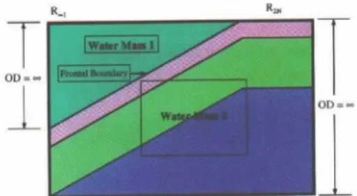
At oceanic fronts the physical structure is usually accompanied by strong gradients in optical properties (Zaneveld and Pak, 1979). The front is modeled as a wedge of homogeneous watermass 1 overlying stratified watermass 2. Figure l shows the structure of the hypothetical front. Referring to equation (12), watermass 1 would have a reflectance of R ~ , if it were infinitely deep, and watermass 2 would have a reflectance of R2N. Note that watermass 2 does not need to be vertically homogeneous. If locations are known where the pure watermasses occur, R=I and R2N can be measured at those locations. Such a location is found for watermass 1 at a distance from the front where the upper layer is thick enough to have b e c o m e optically infinitely deep. It can be

R®~ R2N

~ o t

Fig. 1: Structure of a hypothetical front.

Watermass 1 is physically homogeneous.

At some distance from the front, the opti- cal depth (OD) of watermass 1 becomes infinitely large. The reflectance R ~ 1 is measured here. The reflectance of the stratified watermass 2 is measured at the other side of the front. For further de- tails, see the text.

shown that when watermass 1 overrides stratified watermass 2 and forces it to subside, the layers are stretched so that they b e c o m e thinner perpendicular to the boundary of the two watermasses, but retain the same thickness in the vertical direction. The R2N that is valid when the layers 2 through N has hori- zontal boundaries is thus also valid for inclined boundaries.

The vertical structure of a front can then be d e t e r m i n e d f r o m optical remote sensing using the f o l l o w i n g approach. The reflectance is measured on either side o f the front at a l o c a t i o n where the reflectance has become constant as a function of distance from the front. This determines parameters R=l and R2N in equation (13). The reflectance is then measured as a function of location across the front. Equation (13) is then applied to determine the optical depth at each location. The actual depth can then be determined if g~ is known. Maritorena et al. (1994) have s h o w n that gl is 1.01 to 1.33 times greater than the downward diffuse attenuation coefficient K d (which in turn is a few p e r c e n t d i f f e r e n t f r o m the total diffuse attenuation coefficient).

Fairly good algorithms for the determination of K(490) from remote sensing exist (Austin, 1981), thus at the

"pure" watermass 1 location the K(490) of the overriding watermass 1 can be determined. With the use of relations b e t w e e n g and K as in M a r i t o r e n a et al. (1994), it is then possible to determine the depth of the interface using equation (13).

Sloping Bottoms

It is interesting to note that the same p r o c e d u r e can be applied to a watermass of varying depth overlying a bottom. In that case R2N is the b o t t o m albedo, and equation (13) can be used to derive bottom depth by the same approach. This m e t h o d was used by Philpot and Ackleson (1981) to experi- mentally determine bottom depth using a known bottom albedo. A similar approach was used by Maritorena et al.

(1994). It does not appear to have been r e c o g n i z e d that R2N and hence the albedo can be determined remotely in very shallow water. If the nature of the bottom and therefore the albedo does not change, the bathymetry can be de- t e r m i n e d entirely by passive remote sensing using an approach very similar to that for fronts, without any a priori knowledge of the bottom albedo. In the bottom case we should measure the reflectance in very shallow water close to shore. This will be reflectance R2N.

The layer 2N thus consists of a thin layer of water and the bottom. Physi- cally homogeneous watermass 1 overlies this layer, and its thickness consti- tutes the bathymetry. The thickness of w a t e r m a s s 1 and the b a t h y m e t r y are then determined in an identical way to that described above. The key here is that no a priori knowledge of the bottom albedo is necessary. The only re- quirement is that for accurate bathymetry the albedo must not change. This method could be of use in inaccessible areas. Tidal range can also be determined in this way.

Internal Waves

It is quite common for internal waves to occur at density interfaces. In that case internal waves will c o n t i n u o u s l y change the depth of a layer, which will modify the reflectance. Such an event was observed at East Sound where the ocean color was seen to change from light whitish green to dark green with a periodicity of minutes. Unfortunately, no time series record was obtained. With the use of equation (12), the dependence of the irradiance reflectance on an internal wave can readily be modeled. Sub- stituting

Azl (t,x) = z2 + A cos(~t + kx), (14) where A is the amplitude, w the fre- quency, and k the wavenumber of the in-

46 OCEANOGRAPHY'Vo1. 11, NO. 1°1998

(4)

ternal wave, into equation (121, leads to the desired relationship:

R(0 J,x) = R<

x (1 - e x p { - 2 g j [z2 + A cos(cot + kx)] }) + ReN e x p { - 2 g l [ z 2

+ A cos(cot + kx)] }. (15) B e c a u s e the a m p l i t u d e a p p e a r s in the e x p o n e n t , t h e r e can be a c o n s i d e r a b l e n o n l i n e a r influence on the r e f l e c t a n c e at the surface.

Inversion of the internal w a v e case is interesting b e c a u s e in this case the layer 2N does not occur at the surface, in con- trast to the frontal case. The amplitude o f the internal w a v e can still be s o l v e d for, h o w e v e r , b e c a u s e the r e f l e c t a n c e RZN d o e s not n e e d to be k n o w n , as w i l l be d e m o n s t r a t e d . W e take l a y e r 2N to con- sist o f the water mass structure from the top o f the i n t e r f a c e on w h i c h the w a v e rides, d o w n w a r d to infinity. A t location, x~, where the w a v e is c l o s e s t to the surface, the depth o f the density and optical i n t e r f a c e on w h i c h the i n t e r n a l w a v e r i d e s is z 2 - A, a n d the r e f l e c t a n c e is R(x 0. A t location x 2, where the w a v e is f u r t h e s t f r o m the s u r f a c e , the d e p t h o f the internal w a v e is z, + A, and the re- f l e c t a n c e is R(x2). A p p l y i n g e q u a t i o n (13) at x I and x 2 a n d s u b t r a c t i n g t h e n gives:

[(z2 + A ) - (z2 - A ) l g j

R ( x 2 ) -- R~j

=-0.5 L R-L- -i 7

R ( x l ) - R ~ I + 0.5 In

R2N -- R~ i

o r

2 A g l = - 0 . 5 In R(x2) - R..I

R ( x l ) - R ~ l 1161 The o p t i c a l a m p l i t u d e o f the internal wave can thus be determined, and the actual a m p l i t u d e can be a p p r o x i m a t e d if gl can be determined via the diffuse attenuation coefficient K.

Discussion

T h e a p p l i c a b i l i t y o f the i n v e r s i o n is b y no means universal and is d e p e n d e n t on several factors. The d i f f e r e n c e in the r e f l e c t a n c e s o f the w a t e r m a s s e s , as in e q u a t i o n (13), m u s t be l a r g e e n o u g h to o b t a i n m e a n i n g f u l results. D i f f e r e n t re- m o t e s e n s i n g i n s t r u m e n t s h a v e v a s t l y d i f f e r e n t s e n s i t i v i t i e s in t e r m s o f d e t e r - mining the reflectances. The error in de- t e r m i n i n g the r e f l e c t a n c e s g r e a t l y influ- e n c e s the a b i l i t y to invert. F i n a l l y , the p a r a m e t e r g~ m u s t be d e t e r m i n e d to obtain the a c t u a l d e p t h . A n e x c e l l e n t d i s - cussion on the d e p e n d e n c e o f this p a r a m - eter on e x t e r n a l l i g h t i n g c o n d i t i o n s and the lOP can be found in Maritorena e t al.

(1994). As stated above, they c o n c l u d e d t h a t K < g~ < 1.32 K. T h i s p a r a m e t e r alone can thus lead to a 15% error if we assume that g~ = 1.16 K.

Further work is n e e d e d to test the ap- p r o a c h o u t l i n e d a b o v e using s a t e l l i t e or aircraft optical r e m o t e sensing. At present, s a t e l l i t e s t y p i c a l l y h a v e p i x e l sizes on the o r d e r o f 1 km, so that they could o n l y be u s e d for the l a r g e s t s c a l e f e a - tures. Aircraft remote sensing would thus be more appropriate for the optical detec- tion o f physical features. It would be use- ful to d e t e r m i n e the optical and p h y s i c a l s t r u c t u r e o f the o c e a n d u r i n g r e m o t e sensing in order to assess the viability o f the approach.

Acknowledgement

This work was supported by the Envi- ronmental Optics branch o f the Office o f N a v a l R e s e a r c h and the O c e a n B i o l - o g y / B i o g e o c h e m i s t r y program o f the Na- tional Aeronautics and Space Administra- tion.

References

Austin, R.W., 1981: Remote sensing of the diffuse attenuation coefficient of ocean water. In:

Proceedings of the 29th Symposium of the AGARD Electromagnetic Wave Propagation Panel. 18-1 to 18-9,

Gordon, H.R., R.C. Smith and J.R.V. Zaneveld, 1979: Introduction to ocean optics. In:

Ocean Optics VI, Proc. SP1E 2118, 14-55.

1989: Dependence of the diffuse reflectance of natural waters on the sun angle.

Limnol. Oeeanogr., 34, 1484-1489,

_ _ , O.B, Brown, R.H. Evans, J.W. Brown, R.C. Smith, K.S. Baker and D.K. Clark, 1988: A semi-analytic radiance model of ocean color. J. Geophvs. Res.. 93D, 10,909-10,924.

_ _ , 1992: Diffuse reflectance of the ocean: influence of nonuniform pigment profile. Appl.

Opt.. 31. 2116-2129.

Jerlov. N.G., 1976: Marine Optics. Elsevier Ocean- ography Series, vol. 14, Elsevier, Amste>

dam, 231 pp,

Maritorena, S,, A. Morel and B. Gentili, 1994: Dif- fuse reflectance of oceanic shallow waters:

influence of water depth and albedo. Limnol.

Oceanagr.. 39, 1689-17113.

Mobley, C.D., B. Gentili, H.R. Gordon, Z. Jim G.W. Kattawar, A. Morel, P, Reinersman, K. Stamnes and R.H. Stavn, 1993: Compari- son of numerical models for computing un- derwater lightfields. Appl. Opt., 32, 7484-7504.

Moore, C., J.R.V. Zaneveld and J.C. Kitchen, 1992: Preliminary results from an in sita spectral absorption meter. In: Oeean Optics XI. G,D. Gilbert, ed. Proc. SPIE 17511, 330-337.

Morel, A., 1988: Optical modeling of upper ocean in relation to its biogemms matter content (case 1 waters). J. Geophys. Rex., 93, 749-768.

_ _ and B. Gentili, 1991: Diffuse reflectance of oceanic waters: its dependence on sun angle as influenced by the molecular scattering contribution. Appl. Opt., 30, 4427-4438.

_ _ and B. Gentili, 1993: Diffuse reflectance of oceanic waters. II. Bidirectional aspects.

Appl. Opt., 32, 68644,879.

Philpot, W.D., 1987: Radiative transfer in stratified waters: a single-scattering approximation for irradiance. AppI. Opt., 26. 4123-4 132.

_ _ . , 1989: Bathymetric mapping with passive multispectral imagery. Appl. Opt., 28,

1569 1578.

_ _ and S. Ackleson, 1981: Remote sensing of optically shallow, vertically inhomogeneous waters: a mathematical model. NASA Con- terence Publication 218& Proceedings fi'om Chesapeake Bay Plume Study Superlht~

1980, Williamsburg. VA.

Preisendorfer, R.W., 1976: Hydrologic Optics (in 6 volumes). Dept. of Commerce, NOAA.

Zaneveld, J.R.V., 1982: Remotely sensed reflectance and its dependence on vertical structure: a theoretical derivation. Appl.

Opt., 21, 4146M150.

., 1995: A theoretical derivation of the dependence of the remotely sensed reflectance on the inherent optical properties. J. Geo- phys. Res.. 100, 13,135-13,142.

_ _ , , J.C. Kitchen and C.C. Moore, 1994: Scat- tering error correction of reflecting tube absorption meters. In: Ocean Optics Xll. S.

Ackleson, ed. Proc. SPIE vol. 2258, 44-55.

_ _ and H. Pak, 1979: Optical and particulate properties at oceanic fronts..L Geophys.

Rex., 4, 7781-7790.

OCEANOGRAPHY*VoI, 11, No. 1-1998 47