Recurrence Relations for Single Moments of Order Statistics from Independent Non-identically Distributed Generalized Inverted Exponential Variables
Z. Al-Saiary
Department of Statistics, King Abdul-Aziz University, Jeddah, Saudi Arabia [email protected]
Abstract: The order statistics (OS) arising from independent non-identically (INID) distributed two parameter Generalized Inverted Exponential (GIE) random variables is discussed in this article. Special cases of the rth OS are considered. The moments of the rth order statistic arising from INID distributed GIE random variables are computed. Graphical representations of the probability density function (pdf) and the cumulative distribution function (cdf) of the rth OS arising from INID GIE distribution are plotted. Finally, some numerical examples are given.
[Z. Al-Saiary. Recurrence Relations of Single Moments of the rth Order Statistics from Independent Non- identically Distributed Generalized Inverted Exponential Variables. Academ Arena 2018;10(4):60-68]. ISSN 1553-992X (print); ISSN 2158-771X (online). http://www.sciencepub.net/academia. 9.
doi:10.7537/marsaaj100418.09.
Key words: Moments, Non-identically Order Statistics, Generalized Inverted Exponential Distribution.
1- Introduction
Generalized Inverted Exponential distribution (GIED) was first introduced by [3], which is a generalized form of the inverted exponential distribution (IED) See: [12] & [15]. The important of
GIED in statistical and reliability was discussed in [3], [5] and [6].
The probability density function pdf of two- parameter GIED is given by
2
1
( )
x1
x, 0, , 0 (1)
f x e e x
x
The cumulative distribution function cdf of two - parameter GIED is given by
( ) 1 1
x, 0, , 0 ( 2 )
F x e x
The maximum likelihood estimation and least square estimation are used in [3] to evaluate the parameters and the reliability of the distribution.
[17] obtained the maximum likelihood and Bayes estimators of the parameters of the GIED in case of the progressive type-II censoring scheme with binomial removals. [13] generalized the two parameter GIED using the quadratic rank transmutation map. He discussed the properties of the GIED, derived the moments and examined the order statistics. Moreover, the maximum likelihood estimators for the parameters is briefly investigated and the information matrix is derived. [16] considered various methods of estimation of the unknown parameters of a generalized inverted exponential distribution from a frequentist as well as Bayesian perspective.
[5] handled the reliability analysis of extended GIED with applications. [6] Considered the four- parameter beta GIED and investigated various properties of the model with graphs.
The motive behind this research is that the study of the order statistics for independent but non- identically variables follows generalized inverted exponential distribution was not previously examined, as well as the recurrence relationships to the single moments of the rth order statistics from this distribution was not previously introduced, in which it is difficult to find a closed form.
In section 2, we obtained the probability density function pdf and the cumulative distribution function cdf of the rth OS arising from INID GIED and their graphical representation at n = 3. Computation of moments of the rth OS of INID random variables arising from GIED are found in section 3,
2- Non-identical order statistics from GIED:
The subject on non-identical order statistics is explained widely in the literature in [1], [2], [7], [8], [9], [10]
and [18] for continuous distributions. Also, in [11 ] for discrete distributions.
From [8], [10] and [18], the pdf & cdf of the rth INID OS written as:
Where
p
denotes the summation over all n! permutations (𝑖1, 𝑖2,…, 𝑖𝑛) 𝑜𝑓 (1, 2, … 𝑛). [8] write it in the form of Permanent as:
1 1
( ) 1 ( ) ( ) 1 ( ) ( 4 )
: ( 1) ! ( )!
r n r
f r n x per F x f x F x
r n r
( ) ( ) 1 ( ) ( 5 )
( ) 1 1
j n
F x n F x F x
r j r p j a i a a j i a
Where
pj
is all permutations of i i
1,
2, , i
n
for(1, , ) n
which satisfyi
1 i
2 i
j and1 2
j j n
i
i
i
. Using Permanent, equation (5) written as1
( ) 1
1( )
( ) 1 , ( 6 )
( ) ! ( )!
( ) 1 ( )
n
i r
n n
i n i
F x F x
F x per x
r i n i
F x F x
For GIE distribution where:
( ) 1 1
xi , 0, 0,
i0 ( 7 )
F x e x
i
2
1
( ) 2 1 i , 0, 0, 0 (8 )
x x
f x x e e x
i i i
If we substituting Eq. (7) and (8) in Eq. (4) and (6) and using Mathematica Program 11, we obtain special cases from pdf and cdf of the first, second & the last order statistic when n = 3 as:
3
1
2 3
1
( )
11 : 3 ( 1 )
i
i i
i
f x e e x
x
x
3
) 3 1
( 1 i
x
x
1
1 1
( ) 1 ( ) ( ) 1 ( ) ( 3 )
: ( -1) ! ( - ) !
a r cr n
i i i
p a c r
f x F x f x F x
r n r n r
1 2 1 1 2 3
3
1
1 2
1 2
2
( 3 1
)
1 3
3 1
1 1
1
( ) 3:
(1 ) (1 )
( ) 1
3
( )
i i
i i
i i
i
i i
i
i i
i i i
f x e
e x x
x e
x
e x
Figure1: Graph of pdf of the first INID OS at
1 0.3 ,
2 0.5,
3 0.7
& { 0.5, 1, 1.5 } From Figure (1), we see that the pdf of the first INID GIED is unimodal for different values of the parameters .
The special cases of cdf when n = 3:
( ) 1 ) 1 2 3
1:3 ( 1 e x
F x
1 2
1 2
1 2
1 ( 1 ) ( 1 )
1 1 2
( 1 ) 2
: ( )
1 2
( )
3 e x e x
x x
e e
F x
1 2 3
( 1 ( 1 ) ) ( 1 ( 1 ) ) ( 1
( ) ( 1 ) )
3:3 x x
F x e e e x
2 4 6 8 10
0.5 1.0 1.5
0.5 1 1.5
Figure 2: Graph of cdf of the first INID OS at
1 0.3 ,
2 0.5,
3 0.7
& { 0.5, 1, 1.5 }
3- The Recurrence Relations of the Single Moments of the rth OS arising from INID GIE Random Variables
In this section, we shall present recurrence relation for the single moments of INID OS arising from Eq. (7) and the theorem of (Barakat & Abdelkader, 2003). See [9].
Theorem 3.1 :
For
1 r n , k 1, 2 ,
1
( 1) 1
( ) (1) ( ) (9)
!( ) 0 0 1
0 1 1 2 1
(
i)
k k
k
i ij j
Ij k k ii k i i k E i i ij n a aj ij t at
Where:( 1) ( 1)
( 1) !
1
t
t
i i
j at
i j t a t a t
Or
( 1)
( 1) ( 1, 1)
1
at j
i j t i t a t i t a t
Proof:
In [9] Barakat & Abdelkader derived the single moments of INID OS and generalize this recurrence relation:
( ) ( 1) 1
( 1) ( ) (10 )
: 1
n j
k j n r
I k
r n j n r n r j
Where:1 2
1
1 0 1
( ) ( ) , 1, 2, , (11)
t j
j k
j i
i i i n t
I k k x G x dx j n
Where
( ) 1 ( ),
t t
i i
G x F x
with i i
1, ,
2, i
n
is a permutation of (1, 2, …, n ) for whichi i i
0 2 4 6 8 10
0.2 0.4 0.6 0.8 1.0
0.5
1
1.5
( ) 1 1 , ( 12 ) 1
1 1 2 0
j it
k x
I k k x e dx
j i i i n t
j
Using this series: See [14]
( 1) ( 1 )
( 1) a!
0
b a
b
b z
z a b a
( 1)
1 ( 1)
( 1) a!
0
a
a
i x
i t t i t e
e x
a a
it
1 1 1
1
1 0 1 1 1
0
( 1)
1 ( 1)
( ) ,
a!
( 1)
0 1
1 1 2 0
( 1) ( 1)
1
( 1) !
1 1 2 0
( 1) ( 1)
( 1) ! ,
(
)
t
i
ij j j
j
j j
a
i
a a x
i
a i
a a x
i
a i j j
i a
j t i e x
k t
Ij k i i i n k x t a a dx
j
k e
k x
a a
i i ij n
e dx
a a
1
1
1 1
1 1
0 0 1
1
( 1)
( 1)
1 1 2 0 1 ( 1) ( 1)
( 1) ,
!
( )
(
)
i ij
j
j j
j j t t t t
i i
a a i i j
a a
x j
t t
k xk
i i i n
j a a
e dx
a
I k
j
( 1)
1 ( 1)
( ( 1) !
0 0 1
1 1 2 1
1 1 )
0
1 ( 1)
( ( 1) ( 1 , 1)
0 0 1
1 1 2 1
1 1 )
0
i a
i j j it t
k a a t a a
i i ij n j it t t
j at x
k t
x e dx
i a
i j j t
k a a t a a
i i ij n j it t it t
j at x
k t
x e dx
Substituting:
1 j
y t at x
1
1 1
1 ( )
0 1 0
( 1) (1)
!( )
1 0
( )
k k k
i
k k
k
j at x j
t y
x k e dx t a t y e dy
j
a t i i k E
t i
i k
From [4],
E
n( z )
called the exponential integral function, which is defined as:1
n
( )
nz
E z y
e y y d
By some arranging, we get (9).
Table 1: Ij ( )k using Eq. (9) when n = 3 j
I ( ) k
j
1 1
3 1
( 1)1( 1)
0 ( 1) ( 1, 1)
1 1 1
( ) ( 1) (1)
1 ( 0 !( ) ) ( )
i k k l
k
l l
a
l a
a
a a
I k k E
i i k i
i k
2
1
2 2 2 2
3 2 3 2
1 2
( 1) ( )
1 2 1 2
0 0 ( 1) ( 1) ( 1, 1) ( 1, 1)
1 2 1 1 1 1
1 2
( 1) ( )
3
1 1 2
0 0 ( 1) ( 1) ( 1, 1) ( 1, 1)
1 2 1 1 1 1
2 ( 1) 1 0
( ) ( 1) (1)
2 ( 0 !( ) ) ( (
i k k
k
k
a
a a
a
a a
a
a a a
a a a a
a a a
a a a a
I k k E
i i k i
i k
2 3 2 2 3 2
1 2 ( )
3 1 2
0 ( 1) ( 1) ( 1, 1) ( 1, 1)
2 1 1
) )
a k
a
a a a
a a a a
3
3
1
1
3
3 1
( 1) ( 1, 1)
1 3
1 2 ( 1)
( )
0 0 0
1 2 3
( ) ( 1) (1)
3 ( 0 !( ) ) ( )
i i
a i
k k
k ai
a a a i
a a
i i i i
i
I k k E
i i k i
i k
Corollary ( 3.2 ):
For the case of a sample from Independent Identically Distributed (IID) random variables having cdf in Eq. (7) the
I
j( ) k
in theorem (3.1) simply reduces to1
( ) ( 1) (1) ( ) (13)
!( ) 0 0 1
0 1
i n
k k
k j
j
I j k k i i i k E a a j t at
j
Where:
( 1) ( 1)
( 1) !
1
t t
j at
i j t a t a t
Or
( 1)
( 1) ( 1, 1)
1
at j
a a
j t t t t t
Table 2: Ij ( )k of IID case using Eq. (13) when n = 3 j
I ( ) k
j
1 1
( 1) ( )
0 ( 1) ( 1, 1)
( ) ( 1) (1)
1 ( 0 !( ) )
ii
i k
k i i
k
i i i i
a a
a
a a
I k k E n
i i k i
i k
2
1 2
2 2
1 2
( 1) ( 1 2)
0 0 ( 1) ( 1) ( 1, 1) ( 1, 1)
1 2 1 1
( ) ( 1) (1)
2 ( 0 !( ) ) ( )
i n k
k
k
a
a a
a
a a
a a a a
I k k E
i i k i
i k
3
3
1
1
3
3
3 1
( 1) ( 1, 1)
1
( 1) ( )
0 0 0
1 2 3
( ) ( 1) (1)
3 0 !( )
( )
( )
i i
i k
k
a
n k
a a a i ai
ai ai i
I k k E
i i k i
i k
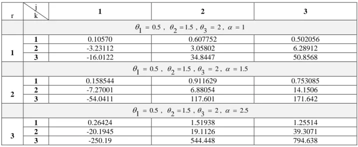
Numerical applications:
The following Table is computed when k = 1, 0.5, 1.5, 2, { 1, 1.5, 2.5 }
2 3
1
Table (3): Ij( )k of INID using Equations in table (1) r
j
k 1 2 3
0.5 , 1.5 , 2 , 1
2 3
1
1
1 0.10570 0.607752 0.502056
2 -3.23112 3.05802 6.28912
3 -16.0122 34.8447 50.8568
0.5 , 1.5 , 2 , 1.5
2 3
1
2
1 0.158544 0.911629 0.753085
2 -7.27001 6.88054 14.1506
3 -54.0411 117.601 171.642
0.5 , 1.5 , 2 , 2.5
2 3
1
3
1 0.26424 1.51938 1.25514
2 -20.1945 19.1126 39.3071
3 -250.19 544.448 794.638
For example, we can compute
1: 3(1) &
2: 3( 2 ) using Eq. (10), Table (1) and Table (2) as:3 (1)
1: 3
I (1)
= 0.26424.2 3
( 2 )
2: 3
I ( 2 ) 2 I ( 2 )
= 6.88054 – 2 (14.1506) = - 21.42066Example (2): Set n = 2,
2 ,
and
1
1 (0.5) 3,
2
1 (0.5) 3 in Theorem (3.1) we get:Table 4: The values of I1(1)arising from INID GIE using Eq. (9) or Table (1)
1
2 1 1.5 2 2.5 31 1.69114 2.11392 0.84557 -0.211392 0.84557
1.5 2.11392 2.53671 1.26835 0.211392 1.26835
2 0.845569 1.26835 0.00000 -1.05696 0.00000
2.5 -0.211392 0.211392 -1.05696 -2.11392 -1.05696
3 0.845569 1.26835 0.00000 -1.05696 0.00000
Conclusion
The order statistics of independent and non- identical distributed random variables is one of the topics that renewed by the emergence of new
References
1. ABDELKADER, Y. (2004) Computing the moments of order statistics from non-identically
non-identically distributed Beta random variables. Stat Pap, 49, 136-149.
3. ABOUAMMOH, A. M. and ALSHINGITI, A.
M. (2009). Reliability estimation of generalized inverted exponential distribution, Journal of Statistical Computation and Simulation, 79(11), 1301–1315.
4. ABRAMOWITZ, M. and STEGUM, I. A.
(1972). Handbook of Mathematical Functions with Formulas, Graphs and Mathematical Tables, 2nd Ed., Dover Publications, New York.
5. ALSHINGITI, A. M., M. KAYID and ALMULHIM, M. (2016), Reliability Analysis of extended generalized inverted exponential distribution with Applications, Journal of Systems Engineering.,27, 484 – 492.
6. BAKOBAN, R. A. and ABU-ZINADAH, H. H
(2017). THE BETA GENERALIZED
INVERTED EXPONENTIAL DISTRIBUTION WITH REAL DATA APPLICATIONS, Volume 15, REVSTAT – Statistical Journal, 65–88.
7. BALAKRISHNAN, N. (1994a) Order statistics from non-identically exponential random variables and some applications. Comput. in Statistics Data-Anal, 18 203-253.
8. BAPAT, R. B. & BEG, M. I. (1989) Order statistics from non-identically distributed variables and permanents. Sankh˜ya, A, 51, 79- 93.
9. BARAKAT, H. & ABDELKADER, Y. (2003) Computing the moments of order statistics from nonidentical random variables Stat Meth Appl, 13, 15-26.
10. DAVID, H. A. & NAGARAJA, H. N. (2003)
Order Statistics, Third Edition. Wiley, New York.
11. Davies, K. and Dembinska, A. (2018).
Computing moments of discrete order statistics from non-identical distributions, Journal of Computational and applied mathematics, 328, 340-345.
12. DURAN, B. S. and LEWIS, T. O. (1989).
Inverted gamma as life distribution, Micro electron. Reliab., 29, 619–626.
13. Elbatal, I. (2013) Transmuted Generalized Inverted Exponential Distribution. DE GRUITER. 28(2):125–133.
14. GRADSHTEYN, I. S. & RYZHIK, I. M. (1980) Table of integrals, series, and products, New York, Academic Press.
15. KELLER, A. Z. and KAMATH, A. R. (1982).
Reliability analysis of CNC Machine Tools, Reliab. Eng. 3, 449–473.
16. SANKU, D. and TANUJIT, D. (2014),
Generalized Inverted Exponential Distribution:
Different Methods of Estimation, American Journal of Mathematical and Management, 33(3).
17. SINGH, S. K., SINGH, U. and KUMAR, M.
(2013). Estimation of Parameters of Generalized Inverted Exponential Distribution for
Progressive Type-II Censored Sample with Binomial Removals, Journal of Probability and Statistics, Volume 2013, Article ID 183652.
http://dx.doi.org/10.1155/2013/183652.
18. VAUGHAN, R. J. & VENABLES, W. N. (1972) Permanent Expressions for Order Statistics Densities. J. R. Statist. Soc, 34, 08 - 10.
4/25/2018