Proceedings of the 2016 Conference on Empirical Methods in Natural Language Processing, pages 1557–1567,
Incorporating Discrete Translation Lexicons into Neural Machine Translation
Philip Arthur
∗, Graham Neubig
∗†, Satoshi Nakamura
∗∗
Graduate School of Information Science, Nara Institute of Science and Technology
†
Language Technologies Institute, Carnegie Mellon University
philip.arthur.om0@is.naist.jp gneubig@cs.cmu.edu s-nakamura@is.naist.jp
Abstract
Neural machine translation (NMT) often makes mistakes in translating low-frequency content words that are essential to understand- ing the meaning of the sentence. We propose a method to alleviate this problem by aug- menting NMT systems with discrete transla- tion lexicons that efficiently encode transla- tions of these low-frequency words. We de- scribe a method to calculate the lexicon proba- bility of the next word in the translation candi- date by using the attention vector of the NMT model to select which source word lexical probabilities the model should focus on. We test two methods to combine this probability with the standard NMT probability: (1) using it as a bias, and (2) linear interpolation. Exper- iments on two corpora show an improvement of 2.0-2.3 BLEU and 0.13-0.44 NIST score, and faster convergence time.1
1 Introduction
Neural machine translation (NMT, §2; Kalchbren- ner and Blunsom (2013), Sutskever et al. (2014)) is a variant of statistical machine translation (SMT;
Brown et al. (1993)), using neural networks. NMT has recently gained popularity due to its ability to model the translation process end-to-end using a sin- gle probabilistic model, and for its state-of-the-art performance on several language pairs (Luong et al., 2015a; Sennrich et al., 2016).
One feature of NMT systems is that they treat each word in the vocabulary as a vector of
1Tools to replicate our experiments can be found at http://isw3.naist.jp/~philip-a/emnlp2016/index.html
Input: I come from Tunisia.
Reference:
チュニジア の 出身です。Chunisia no shusshindesu.
(I’m from Tunisia.)
System:
ノルウェー の 出身です。Noruue- no shusshindesu.
(I’m from Norway.)
Figure 1: An example of a mistake made by NMT on low-frequency content words.
continuous-valued numbers. This is in contrast to more traditional SMT methods such as phrase-based machine translation (PBMT; Koehn et al. (2003)), which represent translations as discrete pairs of word strings in the source and target languages. The use of continuous representations is a major advan- tage, allowing NMT to share statistical power be- tween similar words (e.g. “dog” and “cat”) or con- texts (e.g. “this is” and “that is”). However, this property also has a drawback in that NMT systems often mistranslate into words that seem natural in the context, but do not reflect the content of the source sentence. For example, Figure 1 is a sentence from our data where the NMT system mistakenly trans- lated “Tunisia” into the word for “Norway.” This variety of error is particularly serious because the content words that are often mistranslated by NMT are also the words that play a key role in determining the whole meaning of the sentence.
In contrast, PBMT and other traditional SMT methods tend to rarely make this kind of mistake.
This is because they base their translations on dis-
crete phrase mappings, which ensure that source
words will be translated into a target word that has
1557
been observed as a translation at least once in the training data. In addition, because the discrete map- pings are memorized explicitly, they can be learned efficiently from as little as a single instance (barring errors in word alignments). Thus we hypothesize that if we can incorporate a similar variety of infor- mation into NMT, this has the potential to alleviate problems with the previously mentioned fatal errors on low-frequency words.
In this paper, we propose a simple, yet effective method to incorporate discrete, probabilistic lexi- cons as an additional information source in NMT (§3). First we demonstrate how to transform lexi- cal translation probabilities (§3.1) into a predictive probability for the next word by utilizing attention vectors from attentional NMT models (Bahdanau et al., 2015). We then describe methods to incorporate this probability into NMT, either through linear in- terpolation with the NMT probabilities (§3.2.2) or as the bias to the NMT predictive distribution (§3.2.1).
We construct these lexicon probabilities by using traditional word alignment methods on the training data (§4.1), other external parallel data resources such as a handmade dictionary (§4.2), or using a hy- brid between the two (§4.3).
We perform experiments (§5) on two English- Japanese translation corpora to evaluate the method’s utility in improving translation accuracy and reducing the time required for training.
2 Neural Machine Translation
The goal of machine translation is to translate a se- quence of source words F = f
1|F|into a sequence of target words E = e
|E|1. These words belong to the source vocabulary V
f, and the target vocabulary V
erespectively. NMT performs this translation by cal- culating the conditional probability p
m(e
i| F, e
i1−1) of the ith target word e
ibased on the source F and the preceding target words e
i1−1. This is done by en- coding the context ⟨ F, e
i1−1⟩ a fixed-width vector η
i, and calculating the probability as follows:
p
m(e
i| F, e
i−11) = softmax(W
sη
i+ b
s), (1) where W
sand b
sare respectively weight matrix and bias vector parameters.
The exact variety of the NMT model depends on how we calculate η
iused as input. While there
are many methods to perform this modeling, we opt to use attentional models (Bahdanau et al., 2015), which focus on particular words in the source sen- tence when calculating the probability of e
i. These models represent the current state of the art in NMT, and are also convenient for use in our proposed method. Specifically, we use the method of Luong et al. (2015a), which we describe briefly here and refer readers to the original paper for details.
First, an encoder converts the source sentence F into a matrix R where each column represents a sin- gle word in the input sentence as a continuous vec- tor. This representation is generated using a bidirec- tional encoder
−
→ r
j= enc(embed(f
j), − → r
j−1)
← − r
j= enc(embed(f
j), ← − r
j+1) r
j= [ ← − r
j; − → r
j].
Here the embed( · ) function maps the words into a representation (Bengio et al., 2003), and enc ( · ) is a stacking long short term memory (LSTM) neural network (Hochreiter and Schmidhuber, 1997; Gers et al., 2000; Sutskever et al., 2014). Finally we con- catenate the two vectors − → r
jand ← − r
jinto a bidirec- tional representation r
j. These vectors are further concatenated into the matrix R where the j th col- umn corresponds to r
j.
Next, we generate the output one word at a time while referencing this encoded input sentence and tracking progress with a decoder LSTM. The de- coder’s hidden state h
iis a fixed-length continuous vector representing the previous target words e
i−11, initialized as h
0= 0. Based on this h
i, we calculate a similarity vector α
i, with each element equal to
α
i,j= sim(h
i, r
j). (2) sim ( · ) can be an arbitrary similarity function, which we set to the dot product, following Luong et al.
(2015a). We then normalize this into an attention vector, which weights the amount of focus that we put on each word in the source sentence
a
i= softmax (α
i). (3) This attention vector is then used to weight the en- coded representation R to create a context vector c
ifor the current time step
c = Ra.
Finally, we create η
iby concatenating the previous hidden state h
i−1with the context vector, and per- forming an affine transform
η
i= W
η[h
i−1; c
i] + b
η,
Once we have this representation of the current state, we can calculate p
m(e
i| F, e
i1−1) according to Equation (1). The next word e
iis chosen according to this probability, and we update the hidden state by inputting the chosen word into the decoder LSTM
h
i= enc(embed(e
i), h
i−1). (4) If we define all the parameters in this model as θ, we can then train the model by minimizing the negative log-likelihood of the training data
θ ˆ = argmin
θ
∑
⟨F, E⟩
∑
i
− log(p
m(e
i| F, e
i−11; θ)).
3 Integrating Lexicons into NMT
In §2 we described how traditional NMT models calculate the probability of the next target word p
m(e
i| e
i1−1, F ). Our goal in this paper is to improve the accuracy of this probability estimate by incorpo- rating information from discrete probabilistic lexi- cons. We assume that we have a lexicon that, given a source word f, assigns a probability p
l(e | f ) to tar- get word e . For a source word f , this probability will generally be non-zero for a small number of transla- tion candidates, and zero for the majority of words in V
E. In this section, we first describe how we in- corporate these probabilities into NMT, and explain how we actually obtain the p
l(e | f) probabilities in
§4.
3.1 Converting Lexicon Probabilities into Conditioned Predictive Proabilities
First, we need to convert lexical probabilities p
l(e | f ) for the individual words in the source sentence F to a form that can be used together with p
m(e
i| e
i−11, F ). Given input sentence F , we can construct a matrix in which each column corre- sponds to a word in the input sentence, each row corresponds to a word in the V
E, and the entry cor- responds to the appropriate lexical probability:
LF =
pl(e= 1|f1) · · · pl(e= 1|f|F|)
... ... ...
pl(e=|Ve||f1)· · · pl(e=|Ve||f|F|)
.
This matrix can be precomputed during the encoding stage because it only requires information about the source sentence F .
Next we convert this matrix into a predictive prob- ability over the next word: p
l(e
i| F, e
i1−1). To do so we use the alignment probability a from Equation (3) to weight each column of the L
Fmatrix:
pl(ei|F, ei1−1) =LFai=
pl(e= 1|f1) · · · plex(e= 1|f|F|)
... ... ...
pl(e=Ve|f1)· · · plex(e=Ve|f|F|)
ai,1
...
ai,|F|
.
This calculation is similar to the way how attentional models calculate the context vector c
i, but over a vector representing the probabilities of the target vo- cabulary, instead of the distributed representations of the source words. The process of involving a
iis important because at every time step i, the lexi- cal probability p
l(e
i| e
i1−1, F ) will be influenced by different source words.
3.2 Combining Predictive Probabilities
After calculating the lexicon predictive proba- bility p
l(e
i| e
i1−1, F ), next we need to integrate this probability with the NMT model probability p
m(e
i| e
i1−1, F ) . To do so, we examine two methods:
(1) adding it as a bias, and (2) linear interpolation.
3.2.1 Model Bias
In our first bias method, we use p
l( · ) to bias the probability distribution calculated by the vanilla NMT model. Specifically, we add a small constant ϵ to p
l( · ), take the logarithm, and add this adjusted log probability to the input of the softmax as follows:
p
b(e
i| F, e
i1−1) = softmax(W
sη
i+ b
s+
log(p
l(e
i| F, e
i1−1) + ϵ)).
We take the logarithm of p
l( · ) so that the values will
still be in the probability domain after the softmax is
calculated, and add the hyper-parameter ϵ to prevent
zero probabilities from becoming −∞ after taking
the log. When ϵ is small, the model will be more
heavily biased towards using the lexicon, and when
ϵ is larger the lexicon probabilities will be given less
weight. We use ϵ = 0.001 for this paper.
3.2.2 Linear Interpolation
We also attempt to incorporate the two probabil- ities through linear interpolation between the stan- dard NMT probability model probability p
m( · ) and the lexicon probability p
l( · ) . We will call this the linear method, and define it as follows:
po(ei|F, ei1−1) =
pl(ei= 1|F, ei1−1) pm(e= 1|F, ei1−1)
... ...
pl(ei=|Ve||F, ei1−1) pm(e=|Ve||F, ei1−1)
[ λ
1−λ ]
,
where λ is an interpolation coefficient that is the re- sult of the sigmoid function λ = sig(x) =
1+e1−x. x is a learnable parameter, and the sigmoid func- tion ensures that the final interpolation level falls be- tween 0 and 1. We choose x = 0 (λ = 0.5) at the beginning of training.
This notation is partly inspired by Allamanis et al. (2016) and Gu et al. (2016) who use linear inter- polation to merge a standard attentional model with a “copy” operator that copies a source word as-is into the target sentence. The main difference is that they use this to copy words into the output while our method uses it to influence the probabilities of all target words.
4 Constructing Lexicon Probabilities In the previous section, we have defined some ways to use predictive probabilities p
l(e
i| F, e
i1−1) based on word-to-word lexical probabilities p
l(e | f ). Next, we define three ways to construct these lexical prob- abilities using automatically learned lexicons, hand- made lexicons, or a combination of both.
4.1 Automatically Learned Lexicons
In traditional SMT systems, lexical translation prob- abilities are generally learned directly from parallel data in an unsupervised fashion using a model such as the IBM models (Brown et al., 1993; Och and Ney, 2003). These models can be used to estimate the alignments and lexical translation probabilities p
l(e | f ) between the tokens of the two languages us- ing the expectation maximization (EM) algorithm.
First in the expectation step, the algorithm esti- mates the expected count c(e | f ) . In the maximiza-
tion step, lexical probabilities are calculated by di- viding the expected count by all possible counts:
p
l,a(e | f) = c(f, e)
∑
˜
e
c(f, ˜ e) ,
The IBM models vary in level of refinement, with Model 1 relying solely on these lexical probabil- ities, and latter IBM models (Models 2, 3, 4, 5) introducing more sophisticated models of fertility and relative alignment. Even though IBM models also occasionally have problems when dealing with the rare words (e.g. “garbage collecting” effects (Liang et al., 2006)), traditional SMT systems gen- erally achieve better translation accuracies of low- frequency words than NMT systems (Sutskever et al., 2014), indicating that these problems are less prominent than they are in NMT.
Note that in many cases, NMT limits the target vocabulary (Jean et al., 2015) for training speed or memory constraints, resulting in rare words not be- ing covered by the NMT vocabulary V
E. Accord- ingly, we allocate the remaining probability assigned by the lexicon to the unknown word symbol ⟨unk⟩:
p
l,a(e = ⟨ unk ⟩| f ) = 1 − ∑
i∈Ve
p
l,a(e = i | f). (5) 4.2 Manual Lexicons
In addition, for many language pairs, broad- coverage handmade dictionaries exist, and it is desir- able that we be able to use the information included in them as well. Unlike automatically learned lexi- cons, however, handmade dictionaries generally do not contain translation probabilities. To construct the probability p
l(e | f ) , we define the set of trans- lations K
fexisting in the dictionary for particular source word f , and assume a uniform distribution over these words:
p
l,m(e | f) = {
1|Kf|
if e ∈ K
f0 otherwise .
Following Equation (5), unknown source words will assign their probability mass to the ⟨ unk ⟩ tag.
4.3 Hybrid Lexicons
Handmade lexicons have broad coverage of words
but their probabilities might not be as accurate as the
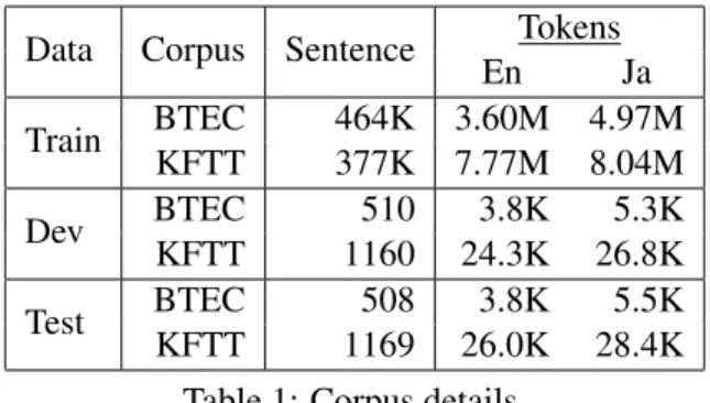
Data Corpus Sentence Tokens
En Ja
Train BTEC 464K 3.60M 4.97M
KFTT 377K 7.77M 8.04M
Dev BTEC 510 3.8K 5.3K
KFTT 1160 24.3K 26.8K
Test BTEC 508 3.8K 5.5K
KFTT 1169 26.0K 28.4K
Table 1: Corpus details.
learned ones, particularly if the automatic lexicon is constructed on in-domain data. Thus, we also test a hybrid method where we use the handmade lexi- cons to complement the automatically learned lexi- con.
2 3Specifically, inspired by phrase table fill-up used in PBMT systems (Bisazza et al., 2011), we use the probability of the automatically learned lex- icons p
l,aby default, and fall back to the handmade lexicons p
l,monly for uncovered words:
p
l,h(e | f ) =
{ p
l,a(e | f) if f is covered p
l,m(e | f ) otherwise (6) 5 Experiment & Result
In this section, we describe experiments we use to evaluate our proposed methods.
5.1 Settings
Dataset: We perform experiments on two widely- used tasks for the English-to-Japanese language pair: KFTT (Neubig, 2011) and BTEC (Kikui et al., 2003). KFTT is a collection of Wikipedia article about city of Kyoto and BTEC is a travel conversa- tion corpus. BTEC is an easier translation task than KFTT, because KFTT covers a broader domain, has a larger vocabulary of rare words, and has relatively long sentences. The details of each corpus are de- picted in Table 1.
We tokenize English according to the Penn Tree- bank standard (Marcus et al., 1993) and lowercase,
2Alternatively, we could imagine a method where we com- bined the training data and dictionary before training the word alignments to create the lexicon. We attempted this, and results were comparable to or worse than the fill-up method, so we use the fill-up method for the remainder of the paper.
3While most words in theVfwill be covered by the learned lexicon, many words (13% in experiments) are still left uncov- ered due to alignment failures or other factors.
and tokenize Japanese using KyTea (Neubig et al., 2011). We limit training sentence length up to 50 in both experiments and keep the test data at the original length. We replace words of frequency less than a threshold u in both languages with the ⟨ unk ⟩ symbol and exclude them from our vocabulary. We choose u = 1 for BTEC and u = 3 for KFTT, re- sulting in | V
f| = 17.8k, | V
e| = 21.8k for BTEC and
| V
f| = 48.2 k, | V
e| = 49.1 k for KFTT.
NMT Systems: We build the described models us- ing the Chainer
4toolkit. The depth of the stacking LSTM is d = 4 and hidden node size h = 800.
We concatenate the forward and backward encod- ings (resulting in a 1600 dimension vector) and then perform a linear transformation to 800 dimensions.
We train the system using the Adam (Kingma and Ba, 2014) optimization method with the default set- tings: α = 1e − 3, β
1= 0.9, β
2= 0.999, ϵ = 1e − 8. Additionally, we add dropout (Srivastava et al., 2014) with drop rate r = 0.2 at the last layer of each stacking LSTM unit to prevent overfitting. We use a batch size of B = 64 and we run a total of N = 14 iterations for all data sets. All of the ex- periments are conducted on a single GeForce GTX TITAN X GPU with a 12 GB memory cache.
At test time, we use beam search with beam size b = 5. We follow Luong et al. (2015b) in replac- ing every unknown token at position i with the tar- get token that maximizes the probability p
l,a(e
i| f
j).
We choose source word f
jaccording to the high- est alignment score in Equation (3). This unknown word replacement is applied to both baseline and proposed systems. Finally, because NMT models tend to give higher probabilities to shorter sentences (Cho et al., 2014), we discount the probability of
⟨ EOS ⟩ token by 10% to correct for this bias.
Traditional SMT Systems: We also prepare two traditional SMT systems for comparison: a PBMT system (Koehn et al., 2003) using Moses
5(Koehn et al., 2007), and a hierarchical phrase-based MT sys- tem (Chiang, 2007) using Travatar
6(Neubig, 2013), Systems are built using the default settings, with models trained on the training data, and weights tuned on the development data.
Lexicons: We use a total of 3 lexicons for the
4http://chainer.org/index.html
5http://www.statmt.org/moses/
6http://www.phontron.com/travatar/
System BTEC KFTT
BLEU NIST RECALL BLEU NIST RECALL
pbmt 48.18 6.05 27.03 22.62 5.79 13.88
hiero 52.27 6.34 24.32 22.54 5.82 12.83
attn 48.31 5.98 17.39 20.86 5.15 17.68
auto-bias 49.74
∗6.11
∗50.00 23.20
†5.59
†19.32 hyb-bias 50.34
†6.10
∗41.67 22.80
†5.55
†16.67
Table 2: Accuracies for the baseline attentional NMT (attn) and the proposed bias-based method using the automatic (auto-bias) or hybrid (hyb-bias) dictionaries. Bold indicates a gain over the attn baseline, † indicates a significant increase at p < 0.05, and ∗ indicates p < 0.10. Traditional phrase-based (pbmt) and hierarchical phrase based (hiero) systems are shown for reference.
proposed method, and apply bias and linear method for all of them, totaling 6 experiments. The first lexicon (auto) is built on the training data using the automatically learned lexicon method of
§4.1 separately for both the BTEC and KFTT ex- periments. Automatic alignment is performed using GIZA++ (Och and Ney, 2003). The second lexicon (man) is built using the popular English-Japanese dictionary Eijiro
7with the manual lexicon method of §4.2. Eijiro contains 104K distinct word-to-word translation entries. The third lexicon ( hyb ) is built by combining the first and second lexicon with the hybrid method of §4.3.
Evaluation: We use standard single reference BLEU-4 (Papineni et al., 2002) to evaluate the trans- lation performance. Additionally, we also use NIST (Doddington, 2002), which is a measure that puts a particular focus on low-frequency word strings, and thus is sensitive to the low-frequency words we are focusing on in this paper. We measure the statistical significant differences between systems using paired bootstrap resampling (Koehn, 2004) with 10,000 it- erations and measure statistical significance at the p < 0.05 and p < 0.10 levels.
Additionally, we also calculate the recall of rare words from the references. We define “rare words”
as words that appear less than eight times in the tar- get training corpus or references, and measure the percentage of time they are recovered by each trans- lation system.
5.2 Effect of Integrating Lexicons
In this section, we first a detailed examination of the utility of the proposed bias method when used
7http://eijiro.jp
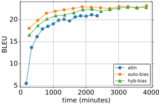
0 1000 2000 3000 4000
time (minutes) 5
10 15 20
BL EU
attnauto-bias hyb-bias
Figure 2: Training curves for the baseline attn and the proposed bias method.
with the auto or hyb lexicons, which empirically gave the best results, and perform a comparison among the other lexicon integration methods in the following section. Table 2 shows the results of these methods, along with the corresponding baselines.
First, compared to the baseline attn, our bias method achieved consistently higher scores on both test sets. In particular, the gains on the more diffi- cult KFTT set are large, up to 2.3 BLEU, 0.44 NIST, and 30% Recall, demonstrating the utility of the pro- posed method in the face of more diverse content and fewer high-frequency words.
Compared to the traditional pbmt systems
hiero, particularly on KFTT we can see that the
proposed method allows the NMT system to exceed
the traditional SMT methods in BLEU. This is de-
spite the fact that we are not performing ensembling,
which has proven to be essential to exceed tradi-
tional systems in several previous works (Sutskever
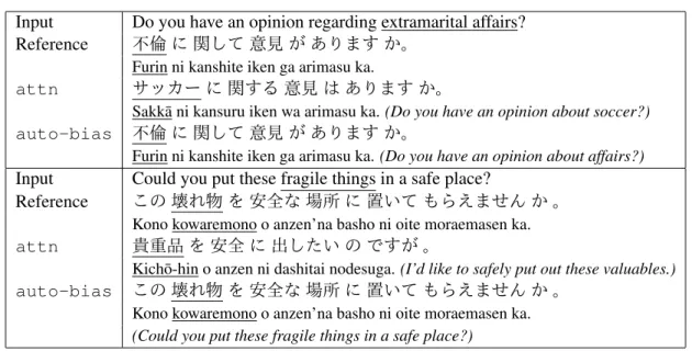
Input Do you have an opinion regarding extramarital affairs?
Reference
不倫 に 関して 意見 が あります か。Furin ni kanshite iken ga arimasu ka.
attn
サッカー に 関する 意見 は あります か。Sakk¯a ni kansuru iken wa arimasu ka.(Do you have an opinion about soccer?)
auto-bias
不倫 に 関して 意見 が あります か。Furin ni kanshite iken ga arimasu ka.(Do you have an opinion about affairs?)
Input Could you put these fragile things in a safe place?
Reference
この 壊れ物 を 安全な 場所 に 置いて もらえません か 。Kono kowaremono o anzen’na basho ni oite moraemasen ka.
attn
貴重品 を 安全 に 出したい の ですが 。Kich¯o-hin o anzen ni dashitai nodesuga.(I’d like to safely put out these valuables.)
auto-bias
この 壊れ物 を 安全な 場所 に 置いて もらえません か 。Kono kowaremono o anzen’na basho ni oite moraemasen ka.
(Could you put these fragile things in a safe place?)
Table 3: Examples where the proposed auto-bias improved over the baseline system attn. Underlines indicate words were mistaken in the baseline output but correct in the proposed model’s output.
et al., 2014; Luong et al., 2015a; Sennrich et al., 2016). Interestingly, despite gains in BLEU, the NMT methods still fall behind in NIST score on the KFTT data set, demonstrating that traditional SMT systems still tend to have a small advantage in translating lower-frequency words, despite the gains made by the proposed method.
In Table 3, we show some illustrative examples where the proposed method (auto-bias) was able to obtain a correct translation while the normal at- tentional model was not. The first example is a mistake in translating “extramarital affairs” into the Japanese equivalent of “soccer,” entirely changing the main topic of the sentence. This is typical of the errors that we have observed NMT systems make (the mistake from Figure 1 is also from attn, and was fixed by our proposed method). The second ex- ample demonstrates how these mistakes can then af- fect the process of choosing the remaining words, propagating the error through the whole sentence.
Next, we examine the effect of the proposed method on the training time for each neural MT method, drawing training curves for the KFTT data in Figure 2. Here we can see that the proposed bias training methods achieve reasonable BLEU scores in the upper 10s even after the first iteration. In con- trast, the baseline attn method has a BLEU score of around 5 after the first iteration, and takes signifi- cantly longer to approach values close to its maximal
Figure 3: Attention matrices for baseline attn and proposed bias methods. Lighter colors indicate stronger attention between the words, and boxes sur- rounding words indicate the correct alignments.
accuracy. This shows that by incorporating lexical probabilities, we can effectively bootstrap the learn- ing of the NMT system, allowing it to approach an appropriate answer in a more timely fashion.
8It is also interesting to examine the alignment vec- tors produced by the baseline and proposed meth-
8Note that these gains are despite the fact that one iteration of the proposed method takes a longer (167 minutes forattn vs. 275 minutes forauto-bias) due to the necessity to cal- culate and use the lexical probability matrix for each sentence.
It also takes an additional 297 minutes to train the lexicon with GIZA++, but this can be greatly reduced with more efficient training methods (Dyer et al., 2013).
(a) BTEC
Lexicon BLEU NIST
bias linear bias linear
- 48.31 5.98
auto 49.74
∗47.97 6.11 5.90 man 49.08 51.04
†6.03
∗6.14
†hyb 50.34
†49.27 6.10
∗5.94
(b) KFTT
Lexicon BLEU NIST
bias linear bias linear
- 20.86 5.15
auto 23.20
†18.19 5.59
†4.61
man 20.78 20.88 5.12 5.11
hyb 22.80
†20.33 5.55
†5.03 Table 4: A comparison of the bias and linear lexicon integration methods on the automatic, man- ual, and hybrid lexicons. The first line without lexi- con is the traditional attentional NMT.
ods, a visualization of which we show in Figure 3. For this sentence, the outputs of both meth- ods were both identical and correct, but we can see that the proposed method (right) placed sharper attention on the actual source word correspond- ing to content words in the target sentence. This trend of peakier attention distributions in the pro- posed method held throughout the corpus, with the per-word entropy of the attention vectors being 3.23 bits for auto-bias, compared with 3.81 bits for attn, indicating that the auto-bias method places more certainty in its attention decisions.
5.3 Comparison of Integration Methods
Finally, we perform a full comparison between the various methods for integrating lexicons into the translation process, with results shown in Table 4.
In general the bias method improves accuracy for the auto and hyb lexicon, but is less effective for the man lexicon. This is likely due to the fact that the manual lexicon, despite having broad coverage, did not sufficiently cover target-domain words (cov- erage of unique words in the source vocabulary was 35.3% and 9.7% for BTEC and KFTT respectively).
Interestingly, the trend is reversed for the linear method, with it improving man systems, but causing decreases when using the auto and
hyb lexicons. This indicates that the linear method is more suited for cases where the lexi- con does not closely match the target domain, and plays a more complementary role. Compared to the log-linear modeling of bias, which strictly en- forces constraints imposed by the lexicon distribu- tion (Klakow, 1998), linear interpolation is intu- itively more appropriate for integrating this type of complimentary information.
On the other hand, the performance of linear in- terpolation was generally lower than that of the bias method. One potential reason for this is the fact that we use a constant interpolation coefficient that was set fixed in every context. Gu et al. (2016) have re- cently developed methods to use the context infor- mation from the decoder to calculate the different in- terpolation coefficients for every decoding step, and it is possible that introducing these methods would improve our results.
6 Additional Experiments
To test whether the proposed method is useful on larger data sets, we also performed follow-up ex- periments on the larger Japanese-English ASPEC dataset (Nakazawa et al., 2016) that consist of 2 million training examples, 63 million tokens, and 81,000 vocabulary size. We gained an improvement in BLEU score from 20.82 using the attn baseline to 22.66 using the auto-bias proposed method.
This experiment shows that our method scales to larger datasets.
7 Related Work
From the beginning of work on NMT, unknown words that do not exist in the system vocabulary have been focused on as a weakness of these sys- tems. Early methods to handle these unknown words replaced them with appropriate words in the target vocabulary (Jean et al., 2015; Luong et al., 2015b) according to a lexicon similar to the one used in this work. In contrast to our work, these only handle unknown words and do not incorporate information from the lexicon in the learning procedure.
There have also been other approaches that incor-
porate models that learn when to copy words as-is
into the target language (Allamanis et al., 2016; Gu
et al., 2016; G¨ulc¸ehre et al., 2016). These models
are similar to the linear approach of §3.2.2, but are only applicable to words that can be copied as- is into the target language. In fact, these models can be thought of as a subclass of the proposed approach that use a lexicon that assigns a all its probability to target words that are the same as the source. On the other hand, while we are simply using a static in- terpolation coefficient λ, these works generally have a more sophisticated method for choosing the inter- polation between the standard and “copy” models.
Incorporating these into our linear method is a promising avenue for future work.
In addition Mi et al. (2016) have also recently pro- posed a similar approach by limiting the number of vocabulary being predicted by each batch or sen- tence. This vocabulary is made by considering the original HMM alignments gathered from the train- ing corpus. Basically, this method is a specific ver- sion of our bias method that gives some of the vocab- ulary a bias of negative infinity and all other vocab- ulary a uniform distribution. Our method improves over this by considering actual translation probabil- ities, and also considering the attention vector when deciding how to combine these probabilities.
Finally, there have been a number of recent works that improve accuracy of low-frequency words us- ing character-based translation models (Ling et al., 2015; Costa-Juss`a and Fonollosa, 2016; Chung et al., 2016). However, Luong and Manning (2016) have found that even when using character-based models, incorporating information about words al- lows for gains in translation accuracy, and it is likely that our lexicon-based method could result in im- provements in these hybrid systems as well.
8 Conclusion & Future Work
In this paper, we have proposed a method to in- corporate discrete probabilistic lexicons into NMT systems to solve the difficulties that NMT systems have demonstrated with low-frequency words. As a result, we achieved substantial increases in BLEU (2.0-2.3) and NIST (0.13-0.44) scores, and observed qualitative improvements in the translations of con- tent words.
For future work, we are interested in conducting the experiments on larger-scale translation tasks. We also plan to do subjective evaluation, as we expect
that improvements in content word translation are critical to subjective impressions of translation re- sults. Finally, we are also interested in improve- ments to the linear method where λ is calculated based on the context, instead of using a fixed value.
Acknowledgment
We thank Makoto Morishita and Yusuke Oda for their help in this project. We also thank the faculty members of AHC lab for their supports and sugges- tions.
This work was supported by grants from the Min- istry of Education, Culture, Sport, Science, and Technology of Japan and in part by JSPS KAKENHI Grant Number 16H05873.
References
Miltiadis Allamanis, Hao Peng, and Charles Sutton.
2016. A convolutional attention network for extreme summarization of source code. InProceedings of the 33th International Conference on Machine Learning (ICML).
Dzmitry Bahdanau, Kyunghyun Cho, and Yoshua Ben- gio. 2015. Neural machine translation by jointly learning to align and translate. InProceedings of the 4th International Conference on Learning Representa- tions (ICLR).
Yoshua Bengio, R´ejean Ducharme, Pascal Vincent, and Christian Janvin. 2003. A neural probabilistic lan- guage model. Journal of Machine Learning Research, pages 1137–1155.
Arianna Bisazza, Nick Ruiz, and Marcello Federico.
2011. Fill-up versus interpolation methods for phrase- based SMT adaptation. In Proceedings of the 2011 International Workshop on Spoken Language Transla- tion (IWSLT), pages 136–143.
Peter F. Brown, Vincent J. Della Pietra, Stephen A. Della Pietra, and Robert L. Mercer. 1993. The mathematics of statistical machine translation: Parameter estima- tion. Computational Linguistics, pages 263–311.
David Chiang. 2007. Hierarchical phrase-based transla- tion. Computational Linguistics, pages 201–228.
Kyunghyun Cho, Bart van Merrienboer, Dzmitry Bah- danau, and Yoshua Bengio. 2014. On the properties of neural machine translation: Encoder–decoder ap- proaches. InProceedings of the Workshop on Syntax and Structure in Statistical Translation (SSST), pages 103–111.
Junyoung Chung, Kyunghyun Cho, and Yoshua Bengio.
2016. A character-level decoder without explicit seg- mentation for neural machine translation. InProceed- ings of the 54th Annual Meeting of the Association for Computational Linguistics (ACL), pages 1693–1703.
Marta R. Costa-Juss`a and Jos´e A. R. Fonollosa. 2016.
Character-based neural machine translation. InPro- ceedings of the 54th Annual Meeting of the Association for Computational Linguistics (ACL), pages 357–361.
George Doddington. 2002. Automatic evaluation of ma- chine translation quality using n-gram co-occurrence statistics. In Proceedings of the Second Interna- tional Conference on Human Language Technology Research, pages 138–145.
Chris Dyer, Victor Chahuneau, and Noah A. Smith.
2013. A simple, fast, and effective reparameterization of IBM model 2. InProceedings of the 2013 Confer- ence of the North American Chapter of the Associa- tion for Computational Linguistics: Human Language Technologies, pages 644–648.
Felix A. Gers, J¨urgen A. Schmidhuber, and Fred A. Cum- mins. 2000. Learning to forget: Continual prediction with LSTM. Neural Computation, pages 2451–2471.
Jiatao Gu, Zhengdong Lu, Hang Li, and Victor O. K. Li.
2016. Incorporating copying mechanism in sequence- to-sequence learning. InProceedings of the 54th An- nual Meeting of the Association for Computational Linguistics (ACL), pages 1631–1640.
C¸aglar G¨ulc¸ehre, Sungjin Ahn, Ramesh Nallapati, Bowen Zhou, and Yoshua Bengio. 2016. Pointing the unknown words. InProceedings of the 54th Annual Meeting of the Association for Computational Linguis- tics (ACL), pages 140–149.
Sepp Hochreiter and J¨urgen Schmidhuber. 1997. Long short-term memory. Neural Computation, pages 1735–1780.
S´ebastien Jean, KyungHyun Cho, Roland Memisevic, and Yoshua Bengio. 2015. On using very large tar- get vocabulary for neural machine translation. InPro- ceedings of the 53th Annual Meeting of the Associa- tion for Computational Linguistics (ACL) and the 7th Internationali Joint Conference on Natural Language Processing of the Asian Federation of Natural Lan- guage Processing, ACL 2015, July 26-31, 2015, Bei- jing, China, Volume 1: Long Papers, pages 1–10.
Nal Kalchbrenner and Phil Blunsom. 2013. Recurrent continuous translation models. InProceedings of the 2013 Conference on Empirical Methods in Natural Language Processing (EMNLP), pages 1700–1709.
Gen-ichiro Kikui, Eiichiro Sumita, Toshiyuki Takezawa, and Seiichi Yamamoto. 2003. Creating corpora for speech-to-speech translation. In8th European Confer- ence on Speech Communication and Technology, EU-
ROSPEECH 2003 - INTERSPEECH 2003, Geneva, Switzerland, September 1-4, 2003, pages 381–384.
Diederik P. Kingma and Jimmy Ba. 2014. Adam: A method for stochastic optimization.CoRR.
Dietrich Klakow. 1998. Log-linear interpolation of lan- guage models. InProceedings of the 5th International Conference on Speech and Language Processing (IC- SLP).
Phillip Koehn, Franz Josef Och, and Daniel Marcu. 2003.
Statistical phrase-based translation. In Proceedings of the 2003 Human Language Technology Conference of the North American Chapter of the Association for Computational Linguistics (HLT-NAACL), pages 48–
54.
Philipp Koehn, Hieu Hoang, Alexandra Birch, Chris Callison-Burch, Marcello Federico, Nicola Bertoldi, Brooke Cowan, Wade Shen, Christine Moran, Richard Zens, Chris Dyer, Ondˇrej Bojar, Alexandra Con- stantin, and Evan Herbst. 2007. Moses: Open source toolkit for statistical machine translation. InProceed- ings of the 45th Annual Meeting of the Association for Computational Linguistics (ACL), pages 177–180.
Philipp Koehn. 2004. Statistical significance tests for machine translation evaluation. InProceedings of the 2004 Conference on Empirical Methods in Natural Language Processing (EMNLP).
Percy Liang, Ben Taskar, and Dan Klein. 2006. Align- ment by agreement. InProceedings of the 2006 Hu- man Language Technology Conference of the North American Chapter of the Association for Computa- tional Linguistics (HLT-NAACL), pages 104–111.
Wang Ling, Isabel Trancoso, Chris Dyer, and Alan W.
Black. 2015. Character-based neural machine transla- tion. CoRR.
Minh-Thang Luong and Christopher D. Manning. 2016.
Achieving open vocabulary neural machine translation with hybrid word-character models. InProceedings of the 54th Annual Meeting of the Association for Com- putational Linguistics (ACL), pages 1054–1063.
Minh-Thang Luong, Hieu Pham, and Christopher D.
Manning. 2015a. Effective approaches to attention- based neural machine translation. InProceedings of the 2015 Conference on Empirical Methods in Natural Language Processing (EMNLP), pages 1412–1421.
Minh-Thang Luong, Ilya Sutskever, Quoc V. Le, Oriol Vinyals, and Wojciech Zaremba. 2015b. Addressing the rare word problem in neural machine translation.
InProceedings of the 53th Annual Meeting of the As- sociation for Computational Linguistics (ACL) and the 7th Internationali Joint Conference on Natural Lan- guage Processing of the Asian Federation of Natural Language Processing, ACL 2015, July 26-31, 2015, Beijing, China, Volume 1: Long Papers, pages 11–19.
Mitchell P Marcus, Mary Ann Marcinkiewicz, and Beat- rice Santorini. 1993. Building a large annotated cor- pus of English: The Penn treebank. Computational Linguistics, pages 313–330.
Haitao Mi, Zhiguo Wang, and Abe Ittycheriah. 2016.
Vocabulary manipulation for neural machine transla- tion. In Proceedings of the 54th Annual Meeting of the Association for Computational Linguistics (ACL), pages 124–129.
Toshiaki Nakazawa, Manabu Yaguchi, Kiyotaka Uchi- moto, Masao Utiyama, Eiichiro Sumita, Sadao Kuro- hashi, and Hitoshi Isahara. 2016. Aspec: Asian scien- tific paper excerpt corpus. InProceedings of the Ninth International Conference on Language Resources and Evaluation (LREC 2016), pages 2204–2208.
Graham Neubig, Yosuke Nakata, and Shinsuke Mori.
2011. Pointwise prediction for robust, adaptable Japanese morphological analysis. In Proceedings of the 49th Annual Meeting of the Association for Com- putational Linguistics (ACL), pages 529–533.
Graham Neubig. 2011. The Kyoto free translation task.
http://www.phontron.com/kftt.
Graham Neubig. 2013. Travatar: A forest-to-string ma- chine translation engine based on tree transducers. In Proceedings of the 51th Annual Meeting of the Associ- ation for Computational Linguistics (ACL), pages 91–
96.
Franz Josef Och and Hermann Ney. 2003. A system- atic comparison of various statistical alignment mod- els. Computational Linguistics, pages 19–51.
Kishore Papineni, Salim Roukos, Todd Ward, and Wei- Jing Zhu. 2002. Bleu: A method for automatic eval- uation of machine translation. InProceedings of the 40th Annual Meeting of the Association for Computa- tional Linguistics (ACL), pages 311–318.
Rico Sennrich, Barry Haddow, and Alexandra Birch.
2016. Improving neural machine translation models with monolingual data. In Proceedings of the 54th Annual Meeting of the Association for Computational Linguistics (ACL), pages 86–96.
Nitish Srivastava, Geoffrey Hinton, Alex Krizhevsky, Ilya Sutskever, and Ruslan Salakhutdinov. 2014.
Dropout: A simple way to prevent neural networks from overfitting. Journal of Machine Learning Re- search, pages 1929–1958.
Ilya Sutskever, Oriol Vinyals, and Quoc V Le. 2014. Se- quence to sequence learning with neural networks. In Proceedings of the 28th Annual Conference on Neural Information Processing Systems (NIPS), pages 3104–
3112.