Toshihiro Kamishima and Jun Fujiki
AIST Tsukuba Central 2, Umezono 1–1–1, Tsukuba, Ibaraki, 305-8568 Japan [email protected],http://www.kamishima.net/
Abstract. We propose a method of using clustering techniques to partition a set of orders. We define the term order as a sequence of objects that are sorted according to some property, such as size, preference, or price. These orders are useful for, say, carrying out a sensory survey. We propose a method called thek-o’means method, which is a modified version of ak-means method, adjusted to handle orders. We compared our method with the traditional clustering methods, and analyzed its characteristics. We also applied our method to a questionnaire survey data on people’s preferences in types of sushi (a Japanese food).
1 Introduction
Clustering is a task to partition a sample set into clusters which have the properties of internal cohesion and external isolation [1], and is a basic tool for exploratory data analysis. Almost all of the traditional methods for clustering are designed to deal with sample sets represented by the attribute vectors or similarity matrices [2]. These cluster- ing methods, therefore, are not suited for handling other types of data. In this paper, we propose a clustering technique for partitioning one such type of data, namely orders.
We define the term order as a sequence of objects that are sorted according to some property. For example, given three objects,x1,x2, andx3, one example of the order is the sequencex3x1x2, which is sorted according to an individual’s preference.
An example in which performing the clustering of orders would be useful would be in completing a questionnaire survey on preferences in foods. The surveyor presents some kinds of foods to each respondent, and requests that he/she sort the foods according to his/her preference. By clustering these preference data, the surveyor would be able to find groups which have the same preference tendency. For such a sensory survey, it is typical to adapt the Semantic Differential (SD) method [3]. In this method, the respondents’ preferences are measured by a scale, the extremes of which are symbolized by antonymous adjectives. For example:
like 5 4 3 2 1 dislike
A proper interpretation of these responses should be, for example, that respondents prefer the objects categorized as “5” to the objects categorized as “4”. However, due to lack of analysis techniques, it is common to assume that all respondents share an understanding of this scale’s range, intervals, and extremes [4]. Such an unrealistic assumption can be avoided by introducing order responses. We therefore developed a clustering technique for orders.
G. Grieser et al. (Eds.): DS 2003, LNAI 2843, pp. 194–207, 2003.
c Springer-Verlag Berlin Heidelberg 2003
We formalize this clustering task in Section 2. Our clustering methods are presented in Section 3. The experimental results are shown in Section 4. Section 5 summarizes our conclusions.
1.1 Related Work
Clustering techniques for partitioning time series data have been previously proposed [5,6,7]. Though both orders and time series data are sequences of observations, there is an important difference between them. The same observations can appear in the same sequences of time series data, but cannot appear in the orders. Therefore, these clustering techniques are not suited for dealing with orders.
The pioneering work of handling orders is Thurstone’s law of comparative judgment [8]. Thurstone proposed a method of constructing a real-value scale from a given set of pairwise precedence information, that indicates which object precedes the other between two objects. Recently, there has been active research in the processing of orders. Cohen et al. [9] and Joachims [10] proposed a method to sort attributed objects associated with pairwise precedence information. Kamishima and Akaho [11] and Kazawa et al. [12]
studied the learning problem from ordered object sets. Mannila and Meek [13] tried to establish the structure expressed by partial orders among a given set of orders. Sai et al.
[14] proposed association rules between order variables. However, since we don’t know of a clustering method for orders, we advocate this new technique in this paper.
2 Clustering Orders
In this section, we formalize a task of clustering orders. An order is defined as a sequence of objects that are sorted according to some property, such as size, preference, or price. An objectxacorresponds to an object, entity, or substance to be sorted. The universal object set,X∗, consists of all possible objects. The order is denoted byO=x1x2 · · · x3. The transitivity is preserved in the same order, i.e., ifx1x2andx2x3thenx1x3. To express the order of two objects,x1x2, we use the sentence “x1 precedesx2.”
Xi ⊆X∗denotes the object set that is composed of all the objects that appear in the orderOi. Let|A|be the size of the setA, then|Xi|is equal to the length of the orderOi. The orderOiis called a full-order ifXi=X∗, and is called a sub-order ifXi⊂X∗.
The task of clustering orders is as follows. A set of sample orders,S ={O1,O2, . . . ,O|S|}is given. Note that it is allowed to beXi=Xj(i=j). In addition, even if x1 x2in the orderOi, it may bex2 x1in the orderOj. The aim of clustering is to divide theSinto a partition. The partition,π={C1,C2,. . . ,C|π|}, is a set of all clusters. Clusters are mutually disjoint and exhaustive, i.e.,Ci∩Cj=∅,∀i,j,i=jand S=C1∪C2∪· · ·∪C|π|. Partitions are generated such that the orders in the same cluster are similar (internal cohesion), and those in the different clusters are dissimilar (external isolation). The similarity measure of orders and our clustering method is presented in the next section.
3 Methods
We modified a well-known clustering algorithmk-means so as to be able to deal with orders. We named this modified method thek-o’means.
3.1 Similarity between Two Orders
To measure the similarity between two orders, we adopted Spearman’s Rank Correlation, which is denoted by “ρ” [15]. Theρis the correlation between ranks of objects. The rank, r(O,x), is the cardinal number that indicates the position of the objectxin the order O. For example, for the orderO=x1x3x2, ther(O,x1)=1and ther(O,x2)=3.
Theρbetween two orders,O1andO2, consisting of the same objects (i.e.,X1=X2) is defined as:
ρ=
x∈X1
r(O1,x)−r¯1
r(O2,x)−¯r2
x∈X1
r(O1,x)−r¯12
x∈X1
r(O2,x)−r¯22, where¯ri= (1/|X1|)
x∈Xir(Oi,x). If no tie in rank is allowed, this can be calculated by the simple formula:
ρ= 1−6×
x∈X1
r(O1,x)−r(O2,x)2
|X1|3− |X1| .
Theρbecomes1if two orders are coincident, and−1if one order is a reverse of the other order. Theρis designed for the two orders consisting of the same objects. In the case of the clustering task in Section 2, the object in one order may not appear in another order. We thus derived the rank correlation from the objects included in both orders, and ignored the rest of the objects. For example, two orders were given:
O1=x1x3x4x6, O2=x5x4x3x2x6.
From these orders, all the objects that were not included in the other orders were elimi- nated. The generated orders were:
O1 =x3x4x6, O2 =x4x3x6. The ranks of objects in these orders were:
r(O1,x3) = 1, r(O1,x4) = 2, r(O1,x6) = 3;
r(O2,x3) = 2, r(O2,x4) = 1, r(O2,x6) = 3. Consequently, theρwas
ρ= 1−6
(1−2)2+ (2−1)2+ (3−3)2 33−3 = 0.5.
Note that if no common objects existed between the two orders, theρ= 0(i.e., no correlation). Over or under estimations in similarities will be caused by this heuristic
of ignoring objects. However, ifXiare randomly sampled fromX∗, the expectation of the observed similarities will be the equivalent to true similarity. Therefore, such over or under estimations can be treated as same as the other types of noises.
To use for the clustering task, distance or dissimilarity is more suitable than similarity.
We defined a dissimilarity between two orders based on theρ:
d(O1,O2) = 1−ρ. (1)
Since the range ofρis[−1,1], this dissimilarity ranges[0,2]. This dissimilarity becomes 0, if two orders are equivalent.
We comment on the reason for adopting Spearman’s ρ as a similarity measure.
Similarities between orders are based on one of the following two quantities. The one is the differences between ranks of objects. The Spearman’sρis an example of this type. The other is the number of discordant object pairs among all object pairs. Formally, an object pair,xaandxb, is discordant ifr(O1,xa)< r(O1,xb)andr(O2,xa)> r(O2,xb), or vice versa. The Kendall’sτis an example of this type. Though the computational complexity of the former quantity is O(|X|), that of the later is O(|X|2). The Spearman’sρcan be calculated faster, so we adopt this as a similarity.
3.2 Order Means
Before describing the algorithm ofk-o’means, we would like to give the definition of an order mean.
In the case ofk-means, the mean of the clusterCis derived such that
¯x= arg min
xi
xj∈C
xi−xj ,
wherexiare data points,Cis a cluster, and · is theL2norm. We extend this notion so as to fit for orders. That is to say, by employing Equation (1) as the loss function, we define an order mean,O¯, as follows:
O¯= arg min
Oj
Oi∈C
d(Oi,Oj). (2) Note that the order mean consists of all objects in all the orders in theC, that isX¯ =
∪Oi∈CXi.
If every order consists of all the objects inX∗(i.e.,Xi=X∗,∀i), the order means are derived by the Borda rule in the 18th century. The rule is equivalent to the following algorithm:
1) For each objectxain theX∗, calculate the following value:
r˜∗(xa) = 1
|C|
Oi∈C
r(Oi,xa). (3) 2) By sorting objects according to the˜r∗(xa)in ascending order, the order mean ofC can be derived.
Note that, if˜r∗(xa) = ˜r∗(xb) , xa=xb, eitherxaxborxbxais allowed.
The proof of the optimality of this algorithm is as follows: First, we relax the limi- tations of ranks. While the strict ranks take one of1 ,. . . ,|X|, the relaxed ranks,r˜(x), are real number and satisfy the condition:
x∈X
r˜(x) = |X|
i=1
i.
Clearly, strict ranks satisfy this condition. Since all the |Xi| are equal, Equation (1) is proportional to the sum of the squared difference between the ranks of two orders.
Therefore, the optimal relaxed ranks can be found by minimizing:
Oi∈C
x∈X∗
(˜r(x)−r(Oi,x))2.
This is minimized at ˜r(x) = ˜r∗(x) ,∀x in Equation (3). We then have to find the strict order,Oj, that minimizes the error. Minimizing the Equation (2) is equivalent to minimizing:
Oi∈C
x∈X∗
r(Oj,x)−r(Oi,x)2
=
Oi∈C
x∈X∗
r(Oi,x)−˜r∗(x))2
+|C|
x∈X∗
r˜∗(x)−r(Oj,x)2
. (4)
Since the first term is already minimized, the strict order meanO¯ corresponds to the strict orderOjthat minimizes the second term. We next show that the order meanO¯is equivalent toO˜∗, that is the order sorted according tor˜∗(x). Assume that there is at least one discordant pair of objects betweenO¯andO˜∗. Formally, there exists an object pair, xaandxb, such that
r˜∗(xa)−r˜∗(xb)
r( ¯O,xa)−r( ¯O,xb)
<0.
Letd1be the second term of the Equation (4) in this case. By swapping these objects only in the order mean, this error becomesd2. Then,
d1−d2=−2|C|(˜r∗(xa)−˜r∗(xb))(r( ¯O,xa)−r( ¯O,xb)
>0.
The fact that the error decreases by swapping objects is contradicted by the assumption that O¯ is an order mean. Therefore, the order mean must not be discordant withO˜∗. Consequently, the above algorithm leads the order mean.
Unfortunately, it is practically a rare situation in which all orders consist of the same object set. If such conditions are not satisfied, the above algorithm cannot be applied. The calculation of the order mean is difficult in this case, since this is a discrete optimization problem. Instead of deriving a strictly optimal solution, we investigated several ad-hoc methods. We tried the methods in [11], such as the one compatible to Cohen’s greedy methods [9]. As a result of the empirical comparisons, we found that the following method based on Thurstone’s model achieved less error in Equation (2) than the others.
The Thurstone’s law of comparative judgment (case V) [8] is the generative model of orders. This model assumes that the scoreR(xa)is assigned to each objectxa. The orders are derived by sorting according to the score. The scores follow the normal distribution, i.e.,R(xa)∼N(µa,σ), whereµais the mean score of the objectxaandσis a common constant standard deviation. Based on this model, the probability that objectxaprecedes thexbis
Pr[xaxb] = ∞
−∞φ(t−µa
σ ) t
−∞φ(u−µb
σ )du dt
=Φ
µa√−µb
2σ
, (5)
whereφ(·)is a normal distribution density function, andΦ(·)is a normal distribution function. Accordingly,
µa−µb=√ 2σΦ−1
Pr[xayb] . Theµa is rescaled intoµ¯a by dividing√
2σ, and the origin is set to the mean ofµ¯1, . . .µ¯|X|¯ , i.e.,
xa∈X¯µ¯a = 0. To estimate these means, Thurstone’s paired comparison method tries to minimize the function:
Q=
xa∈X¯
xb∈X¯
Φ−1
Pr[xaxb]
−(¯µa−µ¯b) 2
.
To minimize theQ, it is differentiated byµ¯a:
∂Q
∂µ¯a=−2
xb∈X¯
Φ−1
Pr[xaxb]
−(¯µa−µ¯b)
=0.
This formula is derived for eachxa=x1,. . . ,x|X|¯. By solving these linear equations, we obtain
µ¯a= 1
|X|¯
xb∈X¯
Φ−1
Pr[xaxb]
. (6)
The order means can be derived by sorting according to theseµ¯a. To derive these values, we have to estimate thePr[xaxb]from the orders in the cluster,C. This probability is estimated by the following process. From the orderOin the cluster, all the object pairs, (xa,xb), are extracted such thatxaprecedesxbin the order. For example, from the order O = x3x1x2, three object pairs,(x3,x1),(x3,x2), and(x1,x2), are extracted.
Such pairs are extracted from all|C|orders in the cluster, and are collected into the set PC. As the probabilityPr[xaxb], we adopted the following Bayesian estimator with Dirichlet prior distribution in order that the probability remains at non-zero:
Pr[xaxb] = |xa,xb|+0.5
|xa,xb|+|xb,xa|+1, where|xa,xb|is the number of the object pairs,(xa,xb), inPC.
Note that, the calculation time for one order mean is O(|X¯|2|C|), since the counting up time for derivingPr[xaxb]is O(|C|
i |Xi|2)≤O(|X|¯ 2|C|), the estimation time of µ¯afor allxa ∈X¯ is O(|X|¯ 2), and the sorting time is O(|X¯|log|X¯|).
Finally, we comment on the method for estimatingµ¯abased on the maximum like- lihood principle (e.g., in [16]). Similar to the originalk-means, ourk-o’means depends on the the initial partition. To cancel this unstable factor, one has to select the best result among a number of trials. The maximum likelihood based method is a kind of gradient decent, so the resultant order also depends on a initial state. More trials are required to cancel this unstable factor. Moreover, since such an iterative method is time-consuming, we adopted the above non-iterative method.
Algorithmk-o’means(S,k,maxIter) S={O1,. . . ,O|S|}: a set of sample orders k: the number of clusters
maxIter: the limit of iteration times
1) initial partition:Sis randomly partitioned intoπ={C1,. . .,Ck},π:=π,t:= 0 2)t:=t+ 1,ift > maxIterthengoto step 6
3)for eachclusterCj∈π, derive the order meansO¯jby the procedure in Section 3.2 4)for eachorderOiinS, assign it to the cluster:arg minCjd( ¯Oj,Oi)
5)ifπ=πthen gotostep 6elseπ:=π,gotostep 2 6)outputπ
Fig. 1. Thek-o’means algorithm
3.3 k-o’means
The k-o’means algorithm is the same as the well-known k-means algorithm, except for the notion of a mean and dissimilarity. The algorithm is shown in Figure 1. First, initial clusters are generated by randomly partitioningS. These clusters are improved by iteratively performing two steps: deriving the order mean for each cluster, and assigning each order to the nearest cluster. If the number of iterations exceeds the threshold or the partitions do not change, the algorithm stops and outputs the current partition. Note that, as the originalk-means algorithm, thek-o’means cannot find the global optimal solution.
Therefore, multiple partitions are derived by starting from different initial partitions, and then selectπminimizing:
Ci∈π
Oj∈Ci
d( ¯Oi,Oj). (7) We here comment on the time complexity of this algorithm. First, the calculation time forkorder means is O(|X∗|2|S|), since one mean is calculated in O(|X|¯ 2|C|) time (see Section 3.2),|C| ≈ |S|/k, and|X¯| ≤ |X∗|. Second, the time for the assignment of one order is O(|Xi|k), because dissimilarity is derived for each of thek clusters and one dissimilarity is calculated in O(|Xi|) time. Thus the total assignment time is O(|S|
i |Xi|k)≤O(|X∗||S|k). Since the number of iteration times is constant, the time
complexity of one iteration is equivalent to the total complexity. Consequently, the total complexity becomes O(|X∗|2|S|+|X∗||S|k). In terms of|S|andk, this is equivalent to that of the originalk-means. However, in terms of|X∗|, the complexity is quadratic.
4 Experiments
We applied ourk-o’means algorithm to two types of data: artificially generated data and real preference survey data. In the former experiment, we compared ourk-o’means and the traditional hierarchical clustering method using the dissimilarity of Equation (1). In addition, by applying thek-o’means to data which had various properties, we revealed the characteristics of this algorithm. In the latter experiment, we analyzed a questionnaire survey data on preferences in sushi (a kind of Japanese food). We used thek-o’means algorithm exploratory tools for analysis. Note that, in the experiments described below, Thurstone’s method is used for deriving the order means sinceXi are always proper subsets ofX∗.
4.1 Evaluation Criteria
Before reporting the experimental results, the evaluation criteria for partitions will be described. In this section, the same object set was divided into two different partitions:
π∗andπˆ. We present two criteria to measure the difference ofπˆfromπ∗.
The first measure is called purity, and is widely used (e.g., in [17]). Assume that the objects in cluster Ci∗ ∈ π∗ are classified into the true class labeledi. If all the objects in theCˆi ∈ πˆclassified into the majority true class, the purity corresponds to the classification accuracy. Formally speaking, the purity is defined as:
purity = 1
|S|
Cˆi∈ˆπ
Cmaxj∗∈π∗|Cˆi∩Cj∗|
. (8)
The range of the purity is[0 , 1], and becomes1if two partitions are identical.
Though this purity is widely used, its lower bound changes according as π∗, and the resulting scale normalization problem makes it difficult to use this as the basis for calculating the means of these criteria. Therefore, we introduce the second criteria, the ratio of information loss (RIL) [18], which is also called the uncertainty coefficient in numerical taxonomy literature. The RIL is the ratio of the information that is not acquired to the total information required for estimating a correct partition. This criterion is defined based on the contingency table for indicator functions [2]. The indicator functionI((xi,xj) ,π)is1if an object pair(xi,xj)are in the same cluster, and0if they are in different clusters. The contingency table is a2×2matrix consisting of elements ast, that are the number of object pairs satisfying the conditionI((xi,xj) ,π∗)=sand I((xi,xj) , ˆπ)=t, among all the possible object pairs. RIL is defined as
RIL = 1
s=0
1
t=0ast
a·· log2aa·t 1 st
s=0as·
a·· log2aa··
s·
, (9)
wherea·t =1
s=0ast,as· =1
t=0ast, anda··=1
s=01
t=0ast. The range of the RIL is[0 , 1], and becomes0if two partitions are identical.
4.2 Experiments on Artificial Data
Data Generation Process. We applied the k-o’means to artificial data in order to compare it with traditional clustering methods and to analyze the method. Test data were generated in the following two steps: In the first step, we generated thekof order means. One random permutation (we called it a pivot) consisting of all objects inX∗ was generated. The otherk−1means were generated by transforming this pivot. Two adjacent objects in the pivot were randomly selected and swapped. This swapping was repeated at specified times. By changing the number of swapping times, the inter-cluster closeness could be controlled.
In the second step, for each of the clusters, its constituent orders were generated.
From the order mean, the |Xi| of the objects were randomly selected. These objects were sorted so as to be concordant with the order mean. Namely, ifxaprecedesxbin the order mean, it should be the case in the generated orders. Again, two adjacent object pairs were randomly swapped. By changing the number of swapping times, the intra-cluster closeness could be controlled.
Table 1. Parameters of experimental data
1) the total number of objects:|X∗|= 100 2) the number of sample orders:|S|= 1000 3) the length of the orders:|Xi|= 10
4) the number of clusters:|π|={2 , 5 , 10 , 50}
5) the swapping times of the order means:{a:∞, b:230000, c:120000}
6) the ratio of the minimum cluster size to the the maximum:{1/1 , 1/2 , 1/5 , 1/10}
7) the swapping times of the sample orders:{a:0 ,b:30 ,c:72}
The parameters of the data generator are summarized in Table 1. The parameters 1–3 are common for all the data.|X∗|and|S|are set so as to be roughly the same as those for the survey data in Section 4.3. If|Xi|is too short, then the differences between orders cannot be tested. However, it is hard for respondents to sort too many objects.
By considering these factors, we set the order length to10. The parameter 4 was the number of clusters. It is difficult to partition if this number is large, since the sizes of the clusters then decrease. The parameter 5 was the swapping time in the first step of the data generation process. Three cases were examined. According to the simulation result, ρmeans between a pivot and the other order means were0.0,0.1, and0.3in the cases ofa,b, andc, respectively. Since the caseawas the most separated, it was the easiest to partition. The parameter 6 controls the deviation of cluster sizes. If the sizes of the clusters are diverged, the relatively small clusters tend to be ignored. Thus,1/10is the hardest to cluster. The last parameter is the swapping times in the second step of the data generation process. The means ofρbetween a sample order and an order mean was1.0, 0.715, and0.442in the cases ofa,b, andc, respectively.ρbetween two random orders
becomes larger than these values with probabilities0.0,0.01, and0.10. Since the case ais the tightest, it was the easiest to partition.
The number of the total parameter combinations was 4×3×4×3=144. For each setting, we generated100sample sets. Below, we will show the means of purity and RIL of these sets.
Table 2. The means of purities and of RIL on artificial data
purity RIL
KOM 0.561 (0.3629) 0.705 (0.4105) AVE 0.466 (0.2966) 0.910 (0.1679) MIN 0.315 (0.2663) 0.999 (0.0014) MAX 0.371 (0.2430) 0.994 (0.0112)
Comparison with Traditional Clustering Methods. We compared our k-o’means algorithm with the traditional hierarchical clustering methods: the minimum distance, maximum distance, and group average methods. Since data are not represented by at- tribute vectors, the originalk-means cannot partition a set of sample orders. However, hierarchical methods can partition a set of sample orders by adopting Equation (1) as dissimilarities between any of the order pairs. We applied ourk-o’means and three tradi- tional algorithms to all144types of artificial data. The correct number of clusters were given as an algorithm’s parameter. The means of purities and RIL are shown in Table 2.
The symbols,KOM,AVE,MIN, andMAXindicate the means derived by thek-o’means, the group average, the minimum distance, and the maximum distance method, respectively.
In parentheses, standard deviations are also shown. Clearly, ourk-o’means is superior to the other three methods. According to the pairedt-test between thek-o’means and each of the other three methods, the difference is significant, even at the significance level of0.1%. We think that this advantage of thek-o’means is due to the following reasons.
The dissimilarity between an order pair tends to be1.0, since common objects are found infrequently. However, ourk-o’means adopted a notion of an order mean. Since order means are derived from far more orders than two, common objects can be found far more frequently. In other words, while the traditional methods are based on only local information, thek-o’means can capture more global features of clusters. In addition, it is well known that a minimum or a maximum are not robust against the outliers, due to effects such as chaining [1].
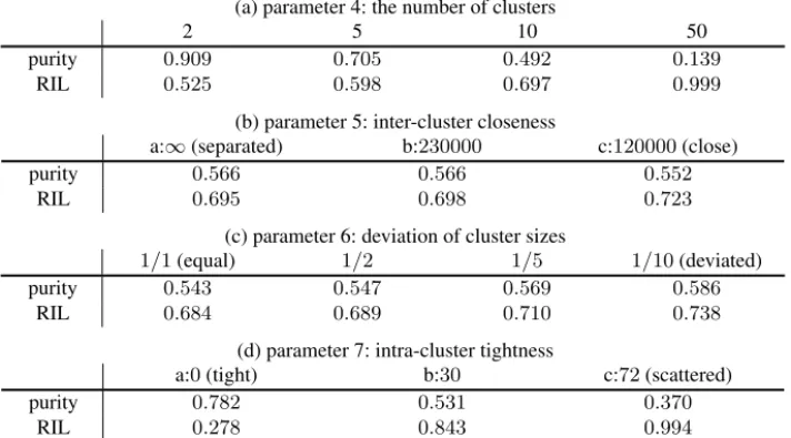
Effects of Data Parameters. We next show the characteristics of thek-o’means ac- cording to the changes of the parameters 4–7 in Table 1. Table 3 shows the means of the purities and of the RIL on each of the data groups that are separated on the specific parameter. For example, in the column labeled “2” in Table 3(a), the means of purities the and of the RIL on 36 types of sample sets whose parameter 4 is 2, i.e.,|π|= 2, are shown. Overall, parameters 4 and 7 affected partitioning, but the others did not. We will next comment on each of these parameters.
Table 3. The means of purities and of RIL on each of the order sets with the same parameters.
(a) parameter 4: the number of clusters
2 5 10 50
purity 0.909 0.705 0.492 0.139
RIL 0.525 0.598 0.697 0.999
(b) parameter 5: inter-cluster closeness
a:∞(separated) b:230000 c:120000(close)
purity 0.566 0.566 0.552
RIL 0.695 0.698 0.723
(c) parameter 6: deviation of cluster sizes
1/1(equal) 1/2 1/5 1/10(deviated)
purity 0.543 0.547 0.569 0.586
RIL 0.684 0.689 0.710 0.738
(d) parameter 7: intra-cluster tightness
a:0(tight) b:30 c:72(scattered)
purity 0.782 0.531 0.370
RIL 0.278 0.843 0.994
Parameter 4: The more the number of clusters increases, the poorer the performance becomes. If the number becomes 50, it is almost impossible to recover the original partition, even in the case of tightest intra-cluster closeness (i.e., the parameter 7 is0).
This can be explained as follows. The number of possible order means can be bounded
|X∗|!. To choose one from these means,log2(|X∗|!)≈525bits information is required.
Roughly speaking, since the number of permutations of|Xi|objects is|Xi|!, one or- der provides log2(|Xi|!) bits information. In total, the orders in one cluster provide
|C|log2(|Xi|!)≈(|S|/|π|) log2(|Xi|!)≈436bits information. Consequently, due to the shortage of information, fully precise order means weren’t derived.
Parameter 5: Closeness between order means does not affect partitioning so much. We don’t know the exact reason, but one possible explanation is that order means can easily be distinguished from each other since they are very long compared to sample orders.
Parameter 6: The originalk-means tends to lead to poor partitions if the sizes of clusters vary, but the k-o’means do not. We think that this is also caused by the above high distinguishablity between order means.
Parameter 7: It is hard to find partitions consisting of clusters in which intra-cluster similarities are low. The sample orders are relatively short, so even a low level of noise affects the partitioning performance a great deal.
4.3 Experiments on Preference Survey Data
We applied ourk-o’means to the questionnaire survey data of preference in sushi. Since notion of true clusters are not appropriate for such a real data, we use thek-o’means as exploratory analysis tools. We asked each respondent to sort 10 objects (i.e., sushi) according to his/her preference. Such a sensory survey is a very suitable area for analysis based on orders. The objects were randomly selected from 100 objects according to
Table 4. Summaries of partition on sushi data
Attributes of Clusters C1 C2
|C|: the numbers of respondents 607 418 A1 : preference to heavy tasting sushi 0.4016 −0.1352 A2 : preference to sushi users infrequently eat −0.6429 −0.6008
A3 : preference to expensive sushi −0.4653 −0.0463
A4 : preference to sushi fewer shops supply −0.4488 −0.2532
their probability distribution, based on menu data from 25 sushi shops found on the WWW. For each respondent, the objects were randomly permutated to cancel the effect of the display order to their responses. The total number of respondents was 1039. We eliminated the data obtained within a response time which was either too short (shorter than 2.5 minutes) or too long (longer than 20 minutes). Consequently, 1025 data was extracted.
We usek-o’means as an exploratory tool, and divided the data into two clusters. The summary of each cluster is shown in Table 4. The results given in the table were the best in terms of Equation (7) among 20 trials. The first row of the table shows the number of respondents grouped into each of the clusters. TheC1is a major cluster. The subsequent four rows show the rank correlation between each order mean and the sorted object list according to the specific object attributes. For example, the fourth row presents theρ between the order mean and the sorted object sequence according to their price. Based on these correlations, we were able to learn what kind of object attributes affected the preferences of the respondents in each cluster. We next comment on each of the object attributes. Note that attributes A1 and A2 were derived from the questionnaire survey by the SD method, and the others from the menu data.
The attribute A1 (the second row) shows whether the object tasted heavy (i.e., high in fat) or light (i.e., low in fat). The positive correlation indicate a preference for heavy tasting. The C1 respondents preferred heavy tasting objects much more than the C2
respondents. The attribute A2 (the third row) shows how frequently the respondent eats the object. The positive correlation indicates a preference for objects that the respondent infrequently eats. Both respondents ofC1 andC2prefer the objects they usually eat.
No clear difference was observed between clusters. The attribute A3 (the fourth row) is the prices of the objects. These were regularized so as to cancel the effects of sushi styles (hand-shaped or rolled), and differences of price between shops. The positive correlation indicate a preference for cheap objects. While theC1respondents preferred expensive objects, theC2respondents did not. The attribute A4 (the fifth row) shows how frequently the objects are supplied at sushi shops. The positive correlation indicates a preference for the objects that fewer shops supply. Though the correlation ofC2is rather larger than that ofC1, the difference is not statistically significant. Roughly speaking, the members of the major groupC1prefer more heavy tasting and expensive sushi than the members of the minor groupC2.
Selecting the number of clusters is worth a mention in passing. Since notion of the optimal number of clusters depend on application of the clustering result, the number cannot be decided in general. However, it can be considered that dividing uniformly
distributed data is invalid. To check this, we tested whether the nearest pair of order means could be distinguished or not. We denote the order means of clusters byO¯1,. . . , ¯O|π|, and that of the entire sample setSbyO¯∗. Letρabbe the rank correlation betweenO¯a
andO¯b, andρ∗abe the rank correlation betweenO¯∗andO¯a. First, we found theO¯αand O¯βsuch that theραβwas the maximum among all pairs of order means. To test whether the closest (i.e. the most correlated) pair of clusters,CαandCβ, should be merged or not, we performed statistical test of the difference between two correlation coefficients, ρ∗αandρ∗β. In this case, the next statistics follows the Studentt-distribution with the degree of freedom|X∗|−3:
t= (ρ∗α−ρ∗β) (|X∗| −3)(1 +ραβ)
2(1−ρ∗α2−ρ∗β2−ραβ2+ 2ρ∗αρ∗βραβ).
If the hypothesisρ∗α=ρ∗β is not rejected, these two clusters should be merged and the number of cluster should be decreased. When partitioning the survey data into two clusters (i.e.k= 2),t = 9.039. At the significance level of1%, it could be concluded that these clusters should not be merged. However, sincet= 1.695whenk= 3, these clusters are invalid and the closest pair of clusters should be merged. Note that any criteria for selecting the number of clusters are not almighty as pointed in [19], since the optimality depends on clustered data and the aim of clustering. For example, when adopting thek-o’means for the purpose of caching [20], the best estimation accuracy was achieved whenkwas larger than two.
5 Conclusions
We developed a clustering technique for partitioning a set of sample orders. We showed that this method outperforms the traditional methods, and presented the characteristics of our method. By using this method, we analyzed a questionnaire survey data on preference in sushi.
The time complexity of the current algorithm is quadric in terms of|X∗|, thus this algorithm is difficult to deal with thousands of objects. We plan to develop the method to accommodate a much larger universal object set.
It is possible to extend our methods to hierarchical ones. We simply embedded the dissimilarity of Equation (1) and the order means to the traditional Ward method.
However, the computation is very slow, since the new order mean cannot be derived from two order means of merged clusters. In addition, the performance was poor. The mean RIL on the artificial data over 10 trials is0.894(compare with Table 2). This is because fully precise order means cannot be derived if the sizes of clusters are small, and the sizes of clusters are very small in the early stage of the Ward method. More elaborate method would be required.
Acknowledgments. A part of this work is supported by the grant-in-aid for exploratory research (14658106) of the Japan society for the promotion of science.
References
1. Everitt, B.S.: Cluster Analysis. third edn. Edward Arnold (1993)
2. Jain, A.K., Dubes, R.C.: Algorithms for Clustering Data. Prentice Hall (1988)
3. Osgood, C.E., Suci, G.J., Tannenbaum, P.H.: The Measurement of Meaning. University of Illinois Press (1957)
4. Nakamori, Y.: Kansei data Kaiseki. Morikita Shuppan Co., Ltd. (2000) (in Japanese).
5. Cadez, I.V., Gaffney, S., Smyth, P.: A general probabilistic framework for clustering individ- uals and objects. In: Proc. of The 6th Int’l Conf. on Knowledge Discovery and Data Mining.
(2000) 140–149
6. Ramoni, M., Sebastiani, P., Cohen, P.: Bayesian clustering by dynamics. Machine Learning 47 (2002) 91–121
7. Keogh, E.J., Pazzani, M.J.: An enhanced representation of time series which allows fast and accurate classification, clustering and relevance feedback. In: Proc. of The 4th Int’l Conf. on Knowledge Discovery and Data Mining. (1998) 239–243
8. Thurstone, L.L.: A law of comparative judgment. Psychological Review 34 (1927) 273–286 9. Cohen, W.W., Schapire, R.E., Singer, Y.: Learning to order things. Journal of Artificial
Intelligence Research 10 (1999) 243–270
10. Joachims, T.: Optimizing search engines using clickthrough data. In: Proc. of The 8th Int’l Conf. on Knowledge Discovery and Data Mining. (2002) 133–142
11. Kamishima, T., Akaho, S.: Learning from order examples. In: Proc. of The IEEE Int’l Conf.
on Data Mining. (2002) 645–648
12. Kazawa, H., Hirao, T., Maeda, E.: Order SVM: A kernel method for order learning based on generalized order statistic. The IEICE Trans. on Information and Systems, pt. 2 J86-D-II (2003) 926–933 (in Japanese).
13. Mannila, H., Meek, C.: Global partial orders from sequential data. In: Proc. of The 6th Int’l Conf. on Knowledge Discovery and Data Mining. (2000) 161–168
14. Sai, Y., Yao, Y.Y., Zhong, N.: Data analysis and mining in ordered information tables. In:
Proc. of The IEEE Int’l Conf. on Data Mining. (2001) 497–504
15. Kendall, M., Gibbons, J.D.: Rank Correlation Methods. fifth edn. Oxford University Press (1990)
16. Hohle, R.H.: An empirical evaluation and comparison of two models for discriminability scales. Journal of Mathematical Psychology 3 (1966) 173–183
17. Huang, Z.: Extensions to thek-means algorithm for clustering large data with categorical values. Journal of Data Mining and Knowledge Discovery 2 (1998) 283–304
18. Kamishima, T., Motoyoshi, F.: Learning from cluster examples. Machine Learning (2003) (in press).
19. Milligan, G.W., Cooper, M.C.: An examination of procedures for determining the number of clusters in a data set. Psychometrika 50 (1985) 159–179
20. Kamishima, T.: Nantonac collaborative filtering: Recommendation based on order responses.
In: Proc. of The 9th Int’l Conf. on Knowledge Discovery and Data Mining. (2003)