Influence of Interlayer Thickness on the Intensity of Singular Stress Field in 3D

and Materials Engineering

Influence of Interlayer Thickness on the Intensity of Singular Stress Field in 3D

Three-Layered Joints under an External Load*

Hideo KOGUCHI** and Masato NAKAJIMA**

**Department of Mechanical Engineering, Nagaoka University of Technology, 1603-1 Kamitomiokamachi, Nagaoka-shi, Niigata, 940-2188, Japan

E-mail:koguchi@mech.nagaokaut.ac.jp Abstract

In the present paper, an influence of interlayer thickness on the singular stress field in 3D adhesive joints with three layers are investigated using eigen analysis formulated by finite element method (FEM) and boundary element method (BEM) using fundamental solutions for two-phase materials. A model for analysis is a three-layered block joint composed of Si, resin and FR-4.5 (Flame Retardant type 4.5, a kind of glass epoxy resin), which constitutes CSP (Chip Size Package) in the electric device. All stress components are expressed as spherical coordinate systems where their origins are located at the vertex of each interface. Firstly, the orders of stress singularity for vertex and lines characterizing singular stress fields are calculated from eigen analysis. Secondly, distributions of stress for the model subjected to an external load are calculated using BEM. Then, the intensity of singularity is derived from these results. Furthermore, 3D intensity of singularity is determined for evaluating a bonding strength in the 3D three-layered bonded joints.

A relationship between the 3D intensity of singularity and the thickness of interlayer is finally examined. It was found that the 3D intensity of singularity becomes a small value when the interlayer thickness reduces, and the 3D intensity of singularity attains an upper limit when the interlayer thickness is larger than the width of the model.

Key words: Boundary Element Method, Stress Singularity, Interface, Adhesive Joint, Eigen Analysis, External Load, Intensity of Singularity, Interlayer Thickness

1. Introduction

A lot of studies about stress singularity occurring at the vertex on the interface in two- and three-dimensional bonded joints have been carried out until now

. Recently, it was found that singular stress field at the vertex has a three-dimensional singularity characteristic accepting an influence of singularity line

. Three-dimensional singular stress field can be expressed using angular function of stress as σ

(r, θ , φ )=K

r

f

( θ , φ ), where r represents the distance from an origin of singular stress field, λ the order of stress singularity, K

the intensity of singularity for stress components σ

, f

( θ , φ ) the angular function considering the influence of singularity line. The order of stress singularity, λ , which characterizes the singular stress field is derived from eigen analysis.

Stress singularity analysis in three-layered joints relating to the recent electric device as CSP (Chip Size Package) was also conducted

. CSP has a structure that IC chip is joined to a substrate with a resin underfill. Recently, the thicknesses of IC chip, resin (interlayer) and substrate are reduced for achieving a high functionality and lightweight. It is important

*Received 16 Nov., 2009 (No. e60) [DOI: 10.1299/jmmp.4.1027]

Copyright © 2010 by JSME

to clarify the influence of material thickness on the singular stress field. In this paper, the influence of interlayer thickness upon the singular stress field in three-dimensional three-layered bonded joints composed of Si (IC chip), resin and FR-4.5 (substrate) is investigated. Firstly, the order of stress singularity is determined from eigen analysis based on FEM (Finite Element Method). Angular function in singular stress field is obtained from eigen vector determined by the eigen analysis. Secondly, stress analysis is conducted using BEM (Boundary Element Method). A model for analysis is three-layered joints subjected to an external load. In this analysis, stress components, σ

, σ

and σ

, which are closely related to the occurrence and growth of crack, are investigated. Combining these results yields the intensity of stress singularity that is a parameter for evaluating the bonding strength of joints. Finally, a three-dimensional intensity of stress singularity is determined for evaluating the strength in the three-dimensional three-layered bonded joints.

Nomenclature

f

( θ , φ ) : Angular function of stress

g

( θ , φ ) : Angular function of stress in BEM analysis

H

: Intensity of stress singularity for φ -direction in BEM analysis K

: Intensity of stress singularity for r-direction, MPa • mm

L

: Intensity of stress singularity for φ -direction in eigen analysis

p : Eigen value

r : Distance from origin, mm t : Thickness of interlayer, mm u : Displacement, mm

W : Width of the model, mm φ : Angle, deg

λ : The order of singularity θ : Angle, deg

ρ : Normalized distance using in eigen analysis σ

: External load, MPa

σ : Stress, MPa

Subscripts

line : on the stress singularity line vertex : in the vertex

i, j : r, θ , φ

2. Analytical formula

2.1 Three-dimensional boundary element method (BEM) Boundary integral equation can be expressed as follows.

c

(P)u

(P) = _∫

{ U

(P,Q)t

(Q) − T

(P,Q)u

(Q) } ^dS(Q) (1) where c

(P) represents a constant depending on the shape of boundary, P and Q are an observation point and a source point locating on the boundary Γ, U

and T

represent the fundamental solutions for displacement and traction. Stress distribution in the domain for analysis is calculated using Hooke’s law and the following equation.

u

(P) = _∫

{ U

(P,Q)t

(Q) − T

(P,Q)u

(Q) } ^dS(Q) (2)

where U

and T

are derivatives of the fundamental solutions of displacement and traction

In this analysis, a mesh division on an interface is not needed, because Rongved’s solution

, which is a fundamental solution for two-phase materials, is used. Hence, the stress distribution on the interface can be calculated accurately. The present analysis model is a three-layered bonded joint, so a domain method is employed in the BEM analysis.

2.2 Eigen analysis method

The order of stress singularity, λ, which characterizes the singular stress field is determined using an eigen equation, which is formulated on the basis of finite element method as follows

.

p

[A] + p[B] + [C]

( ) ^{{ } u =} 0 (3) where λ =Re(p)-1, p is a root of Eq.(3), [A], [B] and [C] are matrices consisting of elastic moduli and the geometry of joints, {u} represents a nodal displacement vector. When -1< λ

<0, a stress singularity exists in the stress field, and when λ >0, the stress singularity disappears.

3. Analysis model and boundary conditions

In the present study, an elastic three-dimensional three-layered block joint which Si and FR-4.5 are joined by resin is analyzed. The model is shown in Fig.1. A quarter model considering the symmetry of the joint is used in BEM analysis. In order to clarify an influence of interlayer thickness on the stress singular field at the vertexes of two interfaces (Si-Resin and Resin-FR-4.5), the thickness of resin, t, is varied from 0.002 to 100mm (t=0.002, 0.004, 0.01, 0.025, 0.1, 0.2, 0.4, 1, 2, 4, 10, 20, 40, 100mm). A unit external load, σ

=1MPa, is applied to the upper surface of Si, and the lower surface of FR-4.5 is fixed in the normal direction to the surface. Eight nodes quadrilateral serendipity element is used, and the minimum length of side in an element near the vertex is 0.01µm×0.01µm. The stresses for spherical coordinate systems with origins at the vertexes of each interface are plotted. Material properties are shown in Table 1, where material property of Si is evaluated as isotropic materials

. In this analysis, stress components σ

, σ

and σ

which are related to the occurrence and growth of crack are investigated.

Fig.1 Model for BEM analysis

4. Results of analysis

4.1 Eigen analysis

4.1.1 Order of stress singularity

A model for eigen analysis is shown in Fig.2, where wedge angles at the stress singularity point O are φ

= φ

=90º, those at a point O

on stress singularity line are φ

= φ

=180º. A mesh division on the developed θ × φ plane used in the eigen analysis is shown in Fig.3. Mesh size of θ and φ coordinates is θ × φ =9º×9º, and an element including the interface and stress singularity lines is equally divided by five, so θ × φ =1.8º×1.8º.

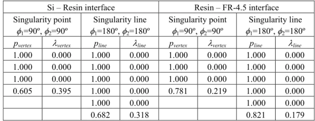
The order of stress singularity at the vertex O, λ

, and that on the singularity line, λ

, for each material combination are shown in Table 2. The order of stress singularity for Si-Resin interface is larger than that for Resin-FR-4.5 interface, and λ

is larger than λ

for each interface. It is found that a triple root of eigen value p=1 at the vertex and a quadruple root of p=1 on the singularity line exist. In the previous study

on the three-dimensional stress singularity, when a triple and quadruple root of p=1 exists, logarithmic singularity may occur at the stress field. Then, the stress field at the vertex can be expressed as follows.

σ

( r ,θ,φ ) ⁼ K

f

( ) θ,φ r

+ K

f

( ) θ,φ ⁺ K

f

( ) θ,φ

k=3

∑

^{( ) ln r}

(4) where N=3 (with a triple root of p=1), N=4 (with a quadruple root of p=1). K

represents the intensity of stress singularity in the r-direction and r = r / t . Here, the angular function f

(θ,φ) of stress σ

can be obtained from eigen vector ({u} on Eq.(3)) corresponding to eigen value p.

4.1.2 Angular functions of stress derived from eigen displacement vector Table 1 Material properties used in analysis

Si Resin FR-4.5

Young’s modulus E, GPa 166.0 2.74 15.34

Poisson’s ratio ν 0.26 0.38 0.15

O O

Material1

Material2

1

2 2 1

Fig.2 A model for eigen analysis

Interface

0 π/2

π/2

π

Resin Silicon

or FR-4.5

Fig.3 A mesh on the developed θ×φ

plane(φ

=φ

=90º)

Spherical coordinate system with an origin located at a vertex of the interface is shown in Fig.4. Where r represents a distance from the origin O to an internal point P, r

represents the radius of sphere. Angular functions of stress in the spherical coordinate system can be obtained from eigen vector corresponding to eigen value, which is shown in Table 2. Eigen displacement in the spherical coordinate system is defined by a normalized distance ρ=r/r

. Angular functions on each interface against angle φ are shown in Figs.5(a) and (b). These figures show the distributions on Si-Resin and Resin-FR4.5 interfaces, respectively. They are normalized by the value of f

(π/2,π/4). It is found that a singular field exists at φ=0º and 90º. Therefore, it is supposed that angular functions are affected depending on the distance from two singularity lines existing at side surfaces. Here, the angular functions of stresses on the interface can be expressed by the following equations.

f

π 2 , φ







 = L

{ ( sin φ )

⁺ ( ^cosφ )

} ^{+ L}

(5) f

π

2 ,φ



 

 = L

{ ( sin φ )

^{cosφ +} ( cos φ )

sin φ }

+ L

{ ( sin φ )

⁺ ( ^cosφ )

} ^{+ L}

^{( sinφ + cos φ )} (6) f

π

2 ,φ



 

 = L

{ ( sin φ )

cosφ − ( cos φ )

sin φ } ^{+ L}

^{( cosφ − sin φ )} (7) where λ

represents the order of stress singularity for the stress singularity line (0≤ λ

≤1). In these equations, 1

term represents the stress singularity because this term is expressed as a term of the – λ

’s powers of sinφ. Hence, it is important to evaluate the coefficient of 1

term, and the coefficient, L

, defines the intensity of stress singularity in the φ-direction.

Table 2 Eigen values and the order of stress singularity for each interface Si – Resin interface Resin – FR-4.5 interface Singularity point

φ

=90º, φ

=90º

Singularity line φ

=180º, φ

=180º

Singularity point φ

=90º, φ

=90º

Singularity line φ

=180º, φ

=180º

p

λ

p

λ

p

λ

p

λ

1.000 0.000 1.000 0.000 1.000 0.000 1.000 0.000 1.000 0.000 1.000 0.000 1.000 0.000 1.000 0.000 1.000 0.000 1.000 0.000 1.000 0.000 1.000 0.000 0.605 0.395 1.000 0.000 0.781 0.219 1.000 0.000

1.000 0.000 1.000 0.000

0.682 0.318 0.821 0.179

x

z

y

O P

r

r

Fig.4 Spherical coordinate system with an origin around a vertex of interface

In these equations, logarithmic terms are neglected. The coefficients, L

, determined by approximating the distributions of angular functions by Eqs.(5)-(7) are shown in Table 3.

4.2 BEM results and intensity of stress singularity

4.2.1 Distribution of stress for r-direction at the vertex of each interface

BEM is used for calculating stress distribution, from which the intensity of stress singularity is determined in the radial direction of the vertex. Distributions of stress, σ

, on each interface against a dimensionless distance r/t at φ=45º are shown in Figs.6(a) and (b) for each thickness of interlayer. Taking the dimensionless distance r/t in the axis of abscissas, stress distributions for various interlayer thicknesses, t, can be arranged, then the range of singular stress field is clearly demonstrated. It is found that the range of singular stress field is r/t<0.4 for the Si-Resin interface, r/t<0.2 for the Resin-FR-4.5 interface.

Magnitude of stress approaches to the value of external load, σ

=1MPa, far from the origin.

Distributions of shear stresses, σ

and σ

, on the interfaces against r/t are shown in Figs.7 and 8. σ

at φ=30º for each interface is plotted, because σ

at φ=45º is zero as shown in Fig.5. In these figures, there is an inflection point in the distribution of σ

in the same location as that of σ

, but there is no point in the distribution of σ

. It is noted that all stress distributions on Si-Resin interface are larger than those on Resin-FR-4.5.

Singular stress field in the three-dimensional joint is represented by Eq.(4). However, the singular stress field is here approximated by using the following equation including t

in K

.

6 5 4 3 2 1 0 -1

90 75 60 45 30 15

0

Si-Resin interface

f

f

f

(a) Si-Resin interface

6 5 4 3 2 1 0 -1

90 75 60 45 30 15

0

Resin-FR-4.5 interface

f

f

f

(b) Resin-FR-4.5 interface Fig.5 Angular function of stress

Table 3 Coefficients of angular functions at each interface

Angular functions Interface L

L

L

λ

Si-resin 0.690 0.000 - 0.318 f

Resin-FR-4.5 0.760 0.000 - 0.179

Si-resin -0.00698 0.643 0.00220 0.318

f

Resin-FR-4.5 -0.00115 0.654 0.0166 0.179

Si-resin 0.0394 0.000 - 0.318 f

Resin-FR-4.5 0.133 0.000 - 0.179

1

0.001 0.01 0.1 1 10

Dimensionless distance r/t

Resin-FR-4.5 interface(φ=45º, θ=90º) Interlayer thickness t, mm

0.002 0.004 0.01

0.025 0.1 0.2 0.4 1 2 4 10 20 40 100

(b) Resin-FR-4.5 interface

Fig.6 Distribution of stress, σ

, against r/t for various thicknesses of interlayer at φ=45º on each interface

1 10

Stress σθθ , MPa

0.001 0.01 0.1 1 10

Dimensionless distance r/t

Si-Resin interface(φ=45º, θ=90º) Interlayer thickness t, mm

0.002 0.004 0.01

0.025 0.1 0.2 0.4 1 2 4 10 20 40 100

(a) Si-Resin interface

0.001 0.01 0.1 1 10

Stress σrθ , MPa

0.01 0.1 1 10

Dimensionless distance r/t Si-Resin interface(φ=45º,θ=90º) Interlayer thickness t, mm

0.002 0.004 0.01

0.025 0.1 0.2 0.4 1 2 4 10 20 40 100

(a) Si-Resin interface

0.01 0.1 1

Stress σrθ , MPa

0.01 0.1 1

Dimensionless distance r/t Resin-FR-4.5 interface(φ=45º, θ=90º) Interlayer thickness t, mm

0.002 0.004 0.01 0.025

0.1 0.2 0.4 1 2 4 10 20 40 100

(b) Resin-FR-4.5 interface

Fig.7 Distribution of stress, σ

, against r/t for various thicknesses of interlayer at φ=45º on each interface

0.01 0.1 1

Stress σφθ , MPa

0.01 0.1 1 10

Dimensionless distance r/t Si-Resin interface(φ=45º, θ=90º) Interlayer thickness t, mm

0.002 0.004 0.01 0.025 0.1 0.2 0.4 1 2 4 10 20 40 100

(a) Si-Resin interface

0.1

Stress σφθ , MPa

0.01 0.1 1

Dimensionless distance r/t Resin-FR-4.5 interface(φ=45º, θ=90º) Interlayer thickness t, mm

0.002 0.004 0.01 0.025 0.1 0.2 0.4 1 2 4 10 20 40 100

(b) Resin-FR-4.5 interface

Fig.8 Distribution of stress, σ

, against r/t for various thicknesses of interlayer at φ=30º

on each interface

σ

r, π 2 ,φ



 

 = K

f

π 2 ,φ



 

 r

+ K

f

π

2 ,φ



 

 (8) where K

t

= K

and the logarithmic term is neglected. Intensity of stress singularity, K

, is determined from the plots shown in Figs.6-8 by a least square method using Eq.(8).

Angular functions f

and f

are normalized by the value at φ=45º on the interface, f

isnormalized by the value at φ=30º on the interface. A relationship between the intensity of singularity in the r-direction, K

, for each interface and the interlayer thickness, t, is shown in Fig.9. It is found that K

is larger than K

and K

. When the thickness of interlayer, t, is larger than 20mm (the same as the width W of the model), K

becomes nearly constant value. It is supposed that an interaction between each interface does not occur in range of t

≥ 20mm. When the thickness of interlayer decreases, then the value of intensity of singularity decreases. Hence, it is supposed that when the thickness of interlayer decreases, the intensity of singularity reduces each other by the interaction. Comparing the distributions on each interface, it is found that the distributions for Si-Resin interface more largely decrease than those for Resin-FR-4.5 interface. Hence, it can be seen that the interaction effect occurs especially in Si-resin interface when Si-Resin and Resin-FR4.5 interfaces approach to each other.

4.2.2 Distribution of stress for φ -direction at the vertex of each interface

In this section, the distributions of stress σ

in the singular stress field on each interface are investigated against φ. It is considered that the stress distribution for φ relates to the angular function of stress obtained from eigen value analysis. However, the singular stress field in BEM is complicatedly influenced from a variation of thickness of interlayer and singularity line. Distributions of stress, σ

, for φ at r=0.0001mm on each interface are shown in Figs.10-12. Stresses increase with increasing the thickness of interlayer, and when the thickness of interlayer is larger than width of the model, W(=20mm), stresses reach an upper limit.

After normalized these distributions, the functions involving in Eq.(8) as well as f

obtained by eigen value analysis can be used. These distributions can be expressed using Eqs.(5)-(7), then the interaction effect attributed to the interlayer thickness and a distance from singularity lines can be evaluated using coefficient L

in Eqs.(5)-(7). Here, the following equations which are different from the angular functions obtained from eigen value analysis are used.

1.4 1.2 1.0 0.8 0.6 0.4 0.2

λ Intensity of singularity K, MPa*mm1ij

0.0

0.01 0.1 1 10 100

Thickness of interlayer t, mm

At Si-Resin interface K_1θθ(φ=45º) K_1rθ(φ=45º) K_1φθ(φ=30º)

At Resin-FR-4.5 interface K1θθ(φ=45º) K1rθ(φ=45º) K_1φθ(φ=30º)

Fig.9 A relationship between the intensity of singularity in the r-direction, K

, on each

interface and interlayer thickness, t

25

20

15

10

5

0

90 75 60 45 30 15

0

Si-Resin interface(r=0.0001mm,θ=90º) Interlayer thickness t, mm 0.002 0.004

0.01 0.025 0.1 0.2 0.4 1 2 4 10 20 40 100

(a) Si-Resin interface

-3.0 -2.5 -2.0 -1.5 -1.0 -0.5 0.0

Stress σrθ , MPa

90 75 60 45 30 15

0

Resin-FR-4.5 interface(r=0.0001mm,θ=90º) Interlayer thickness t, mm 0.002 0.004

0.01 0.025 0.1 0.2 0.4 1 2 4 10 20 40 100

(b) Resin-FR-4.5 interface Fig.11 Distribution of stress, σ

, against φ at r=0.0001mm for various thicknesses of

interlayer on each interface

100 90 80 70 60 50 40 30 20 10 0

90 75 60 45 30 15

0

, deg

Si-Resin interface (r=0.0001mm,θ=90º) Interlayer thickness t, mm

0.002 0.004 0.01

0.025 0.1 0.2 0.4 1 2 4 10 20 40 100

(a) Si-Resin interface

16 14 12 10 8 6 4 2 0

90 75 60 45 30 15

0

, deg

Resin-FR-4.5 interface (r=0.0001mm,θ=90º) Interlayer thickness t, mm

0.002 0.004 0.01

0.025 0.1 0.2 0.4 1 2 4 10 20 40 100

(b) Resin-FR-4.5 interface Fig.10 Distribution of stress, σ

, against φ at r=0.0001mm for various thicknesses of

interlayer on each interface

-32 -24 -16 -8 0 8 16 24 32

Stress σφθ , MPa

90 75 60 45 30 15

0

Si-Resin interface (r=0.0001mm,θ=90º) Interlayer thickness t, mm

0.002 0.004 0.01

0.025 0.1 0.2 0.4 1 2 4 10 20 40 100

(a) Si-Resin interface

-4 -3 -2 -1 0 1 2 3 4

Stress σφθ , MPa

90 75 60 45 30 15

0

Resin-FR-4.5 interface (r=0.0001mm,θ=90º) Interlayer thickness t, mm

0.002 0.004 0.01

0.025 0.1 0.2 0.4 1 2 4 10 20 40 100

(b) Resin-FR-4.5 interface Fig.12 Distribution of stress, σ

, against φ at r=0.0001mm for various thicknesses of

interlayer on each interface

g

π 2 ,φ



 

 = H

{ ( sinφ )

⁺ ( ^cosφ )

} ^{+ H}

(9) g

π

2 ,φ



 

 = H

{ ( sin φ )

cos φ + ( cosφ )

^sinφ }

+ H

{ ( sin φ )

⁺ ( ^cosφ )

} ^{+ H}

^{( sin φ + cosφ )} (10) g

π

2 ,φ



 

 = H

{ ( sin φ )

cosφ − ( cosφ )

sinφ } ^{+ H}

^{( cos φ − sinφ )} (11) where g

represents the stress normalized by the value at r=0.0001mm, φ=30º(σ

) or 45º(σ

and σ

) and θ=90º, which is a function of angle φ on the interface, and the intensity of singularity in the φ-direction, L

, is written as H

. f

does not include the influence of interaction which occurs when each interface approaches to each other, because f

is calculated from eigen vector for two-phase material with an interface. Hence, it is important to evaluate g

including the interaction effect. The coefficients, H

, determined by approximating the distributions of normalized stress shown in Figs.10-12 by Eqs.(9)-(11) are demonstrated in Fig.13. It is found that H

is the largest value, next H

, and H

is the smallest value. H

does not vary with the interlayer thickness, t. Comparing these with the value of Table 3, H

of each stress component are near to L

.

4.2.3 Three-dimensional intensity of stress singularity

Three-dimensional singular stress field on the interface in the bonded joint can be expressed by using Eqs.(9)-(11) as follows.

σ

r, π 2 ,φ



 

 = K

g

π 2 ,φ



 

 r

+ K

g

π

2 ,φ



 

 (12) Here, substituting the angular functions of Eqs.(9)-(11) into Eq.(12), then the three-dimensional intensity of singularity can be derived by combining the intensity of singularity in the r-and φ-directions, K

and H

, as follows.

σ

r, π 2 ,φ



 

 = K

( sin φ )

⁺ ( cos φ )

^{+ H}

H

 



 

 r

+ K

g

(13)

-1.0 -0.8 -0.6 -0.4 -0.2 0.0 0.2 0.4 0.6 0.8 1.0

Intensity of stress singularity in theφ-direction

0.01 0.1 1 10 100

Thickness of interlayer t, mm Si-Resin interface

H1θθ H1rθ H1φθ

Results of Eigen Analysis L1θθ L1rθ L1φθ

(a) Si-Resin interface

Fig.13 A relationship between intensity of singularity in the φ-direction on each interface and interlayer thickness, t

-1.0 -0.8 -0.6 -0.4 -0.2 0.0 0.2 0.4 0.6 0.8 1.0

Intensity of stress singularity in theφ-direction

0.01 0.1 1 10 100

Thickness of interlayer t, mm Resin-FR-4.5 interface

H_1θθ H_1rθ H_1φθ Results of Eigen Analysis

L1θθ L1rθ L1φθ ( - L1φθ

)

(b) Resin-FR-4.5 interface

σ

r, π 2 , φ



 

 = K

sin φ

( )

cos φ + ( cos φ )

sin φ + H

H

{ ( sin φ )

⁺ ( cos φ )

}

+ H

H

( sin φ + cos φ )





 





 







 





 



r

+ K

g

(14)

σ

r, π 2 , φ



 

 = K

sin φ

( )

cos φ − ( cos φ )

sin φ + H

H

( cos φ − sin φ )



 

 



 

  r

+ K

g

(15) where coefficients, K

=K

H

, are used to evaluate the three-dimensional intensity of stress singularity. A relationship between K

on each interface and interlayer thickness, t, is shown in Fig.14. It is found that the distribution of K

follows the distribution of K

(as shown in Fig.9) because the intensity of singularity in the φ -direction, H

, is nearly constant against the interlayer thickness. Figure 14 demonstrates the existence of an upper limit of the three-dimensional intensity of singularity, K

, when the thickness of interlayer is equal to the width of the model, as well as K

. Furthermore, it is found that K

for σ

is especially larger than that for another shear stress components. Therefore, it is supposed that when the bonding strength in the bonded joints like as Fig.1 is estimated by the intensity of stress singularity, shear stress components may be neglected, and only component of normal stress to the interface is enough to evaluate the strength of joints.

5. Conclusions

Singular stress analysis in the three-layered block joints was conducted for various values of interlayer thickness under an external tensile load. Finally, a relationship between three-dimensional intensity of stress singularity and interlayer thickness was investigated.

Results are summarized as follows.

(1) The intensity of stress singularity in the r-direction, K

, decreased with decreasing the thickness of interlayer owing to the interaction of the upper (Si-Resin) and the lower (Resin-FR-4.5) interfaces. When the thickness of interlayer is equal to the width of model, the interaction of each interface vanished, and then the intensity of singularity reached an upper limit.

(2) The intensity of stress singularity in the φ -direction, H

, was not affected by the interlayer thickness. The value was near to the value of L

in the angular function derived

1.0 0.9 0.8 0.7 0.6 0.5 0.4 0.3 0.2 0.1 0.0 -0.1

0.01 0.1 1 10 100

Thickness of interlayer t, mm

Silicon-Resin interface K_1θθ^3D K_1rθ^3D K_1φθ^3D Resin-FR-4.5 interface

K1θθ3D K1rθ3D

K1φθ3D

Fig.14 A relationship between three-dimensional intensity of singularity, K

, on each

interface and interlayer thickness, t

from eigen value analysis.

(3) Three-dimensional intensity of stress singularity, K

, was obtained combining the intensity of singularity in the r- and φ -directions. K

varied with the interlayer thickness in a similar to K

, because H

were nearly constant against the interlayer thickness.

(4) Only normal stress σ

of K

might relate to the failure of the three-dimensional bonded joints under a tensile load in the perpendicular direction of the interface, because another shear stresses were very small.

References

(1) Bogy, D.B., On the Problem of Edge-Bonded Elastic Quarter Planes Loaded at the Boundary, International Journal of Solids Structures, Vol.6, (1970), pp.1287-1313.

(2) Bogy, D.B., Two Edge-Bonded Elastic Wedges of Different Materials and Wedge Angles under Surface Tractions, Journal of Applied Mechanics, Vol.38, (1971), pp.377-386.

(3) Bogy, D.B. and Wang, K.C., Stress Singularities at Interface Corners in Bonded Dissimilar Isotropic Elastic Materials, International Journal of Solids Structures, Vol.7, (1971), pp.993-1005.

(4) Dempsey, J.P. and Sinclair, G.B., On the Stress Singularities in the Plane Elasticity of the Composite Wedge, Journal of Elasticity, Vol.9, (1979), pp.373-391.

(5) Munz, D. and Yang, Y.Y., Stress Singularity at the Interface in Bonded Dissimilar Materials Under Mechanical and Thermal Loading, Journal of Applied Mechanics, Vol.59, (1992), pp.857-861.

(6) Munz, D., Matthias, A. and Yang, Y.Y., Thermal Stresses in Ceramic-Metal Joints with an Interlayer, Journal of the American Ceramic Society, Vol.78, No.2(1995), pp.285-290.

(7) Ioka, S., Masuda, K. and Kubo, S., Singular Stress distributions near the Edge of Interface of Bonded Dissimilar Materials with an Interlayer, Journal of Society Material Science, Japan, Vol.53, No.8(2004), pp.841-845.

(8) Inoue, T., Koguchi, H. and Yada, T., Basic Characteristic on Distribution of Thermal Stresses near Apex in Dissimilar Materials, Transactions of the Japan Society of Mechanical Engineers, Series A, Vol.61, No.581(1995), pp.73-79.

(9) Koguchi, H., Fujimagari, M., Analysis for The Order of Stress Singularity, Displacement and Stress Fields at A Vertex of Three-Dimensional Joints in Electric Devices, Transactions of the Japan Society of Mechanical Engineers, Series A, Vol.67, No.656(2001), pp.595-602.

(10) Koguchi, H., Sakai, H. and Prukvilailert, M., Analysis of Stress Singularity Field in Three-Dimensional Joints Using Three-Dimensional Boundary Element Method, Transactions of the Japan Society of Mechanical Engineers, Series A, Vol.71, No.703(2005), pp.402-410.

(11) Koguchi, H. et al., Analysis of Stress Singularity Fields in Three-Dimensional Joints by Three-Dimensional Boundary Element Method Using Fundamental Solution for Two-Phase Transversely Isotropic Materials, Transactions of the Japan Society of Mechanical Engineers, Series A, Vol.69, No.679(2003), pp.585-593.

(12) Koguchi, H. and Taniguchi, T., Characteristics of Stress Singularity Field of residual Thermal Stresses at Vertex in Three-Dimensional Bonded Joints, Transactions of the Japan Society of Mechanical Engineers, Series A, Vol.74, No.724(2008), pp.864-872.

(13) Koguchi, H. and Konno, N., Intensity of Residual Thermal Stresses at the Vertex in Three-Dimensional Joints with Three-Layers(Influence of Thickness of Interlayer), Society of Mechanical Engineers, Series A, Vol.75, No.757(2009), pp.1148-1155.

(14) Rongved, L., Force Interior to One of Two Jointed Semi-Infinite Solid, Proceedings Second Midwestern Conference on Solid Mechanics, (1995), pp.1-13.

(15) Pageau, S.S. and Bigger, Jr S.B., Finite Element Evaluation of Free-Edge Singular Stress

Fields in Anisotropic Material, International Journal of Numerical Methods in Engineering, Vol.38, (1995), pp.2225-2239.

(16) Haiss, W., Surface Stress of Clean and Adsorbate-Covered Solids, Reports on Progress in

Physics, Vol.64, No.5(2001), pp.591-648.