Sparse DP Quantization Algorithm

(1)

PAPER

Sparse DP Quantization Algorithm

Yukihiro BANDOH^†a), Seishi TAKAMURA^†,andAtsushi SHIMIZU^†,Senior Members

SUMMARY We formulate the design of an optimal quantizer as an optimization problem that finds the quantization indices that minimize quantization error. As a solution of the optimization problem, an approach based on dynamic programming, which is called DP quantization, is proposed. It is observed that quantized signals do not always contain all kinds of signal values which can be represented with given bit-depth. This property is called amplitude sparseness. Because quantization is the amplitude dis- cretization of signal value, amplitude sparseness is closely related to quantizer design. Signal values with zero frequency do not impact quantization error, so there is the potential to reduce the complexity of the optimal quantizer by not computing signal values that have zero frequency. However, conventional methods for DP quantization were not designed to consider amplitude sparseness, and so fail to reduce complexity. The proposed algorithm offers a reduced complexity optimal quantizer that minimizes quantization error while addressing amplitude sparseness. Experimental results show that the proposed algorithm can achieve complexity reduction over conventional DP quantization by 82.9 to 84.2% on average.

key words: quantization, sparseness, dynamic programming

1. Introduction

The purpose of quantization [1] is to generate codewords (quantization indices) based on a given metric. The design of the optimal quantizer leads to a kind of minimization problem, that is, how to generate the quantization indices that can minimize a distortion (quantization error) caused by a quantization process. A typical form of quantization error is summation of square error (SSE). Quantization schemes are classified into two types: conversion from continuous signal to discrete one, and conversion from fine discrete signal to coarse discrete one. This manuscript focuses on the latter type. The latter type is a kind of bit depth conversion, and is required for display adaptation[2],[3], bit-depth scalable coding[4],[5]and HDR video coding[6].

The approaches proposed to solve the above-mentioned minimization problem fall into two types: analytical optimization (which calculates the optimal solution analytically) and numerical optimization (which uses numerical computation). If the probability density function (PDF) of quantized data can be represented in particular parametric- form, for example, a uniform distribution, Gauss distribution or Laplace distribution, analytical optimization can be adopted where the codewords for symbols generated from these PDFs are analytically optimizes. However, the PDF

Manuscript received May 23, 2018.

Manuscript revised October 27, 2018.

†The atuthors are with NTT Media Interigence Laboratories, NTT Corporation, Yokosuka-shi, 239-0847 Japan.

a) E-mail: [email protected] DOI: 10.1587/transfun.E102.A.553

of real quantized data generally can not be represented in the desired parametric forms. Therefore, such analytical optimization approaches generally cannot generate optimal quantizers for real data.

Consequently, numerical optimization approaches, which do not require any particular parametric form of PDF are more common. Typical of this result is the Lloyd- Max quantization algorithm (hereafter LM quantization) [7],[8], which generates quantization indices and boundaries of quantization bins iteratively, until a given convergence condition is satisfied.

However, two problems with this algorithm have been pointed out. First, LM quantization can not guarantee the optimal solution. This is because the algorithm is designed based on a necessary condition for optimal quantization.

LM quantization can generate the optimal solution, only if the logarithm function of the PDF for quantized data offers convexity. For example, the above convexity condition is satisfied if the PDF follows a uniform distribution, Gauss distribution or Laplace distribution. On the other hand, when the quantized data does not satisfy the convexity condition, the most common case, LM quantization may fall into local minimum. It depends on the initial codewords as to whether LM quantization yields the optimal solution or not. Note that no specific strategy has been adopted for optimizing initial codewords. Second, the computation complexity of LM quantization can not be evaluated. This is because the algorithm is based on an iterative process and its convergence depends on the initial codewords.

In order to design optimal quantizers, adaptive quantization algorithms based on dynamic programming (henceforth, abbreviated to DP quantization) have been studied.

Bruce [9] applied the principle of optimality in dynamic programming to optimizing quantizer, and showed that the complexity associated with designing an optimizing quantizer can be reduced from exponential time to polynomial time. Sharma[10]proposed a low complexity algorithm for designing a DP quantizer that minimizes the quantization error subject to convexity constraint. Wu[11]proposed an algorithm to reduce the complexity of optimal path finding in DP quantization using matrix search.

As a kind of the above-mentioned quantization, bit- depth conversion (BDC) is used in image processing. BDC transforms the bit-depth of input signal and generates signal with lower bit-depth. For example, BDC is used to adjust high bit-depth signal to legacy displays which do not support high bit-depth signal. Furthermore, BDC plays an impor- Copyright c2019 The Institute of Electronics, Information and Communication Engineers

(2)

tant role in bit-depth scalable codec[4],[5],[12],[13]as a key process for generating a layer-structured data that con- sists of a base layer and enhancement layers. BDC separates an input signal of the encoder into signal for the base layer and those for enhancement layers. The base layer is con- structed to have backward compatibility to a decoder that does not support high bit-depth signal.

When designing optimal quantizers for image signals, it is important to note that most image signals feature amplitude sparseness of signal value, that is, pixel value. In other words, the signal values do not fully utilize the given bit-depth. For example, if an image whose bit-depth is 10 bits exhibits sparseness, it contains fewer than 1024 signal values, although the bit-depth can represent up to 1024 signal values. Some studies on image coding report that coding efficiency can be improved by considering amplitude sparseness. Lossless coding algorithms[14],[15]and a near-lossless coding algorithm[16]improve coding efficiency by utilizing fewer pixel values for images with amplitude sparseness.

The histogram of an image with sparseness has some insignificant elements, that is, their frequency is zero (hereafter called zero-frequency). Signal values that have zero- frequency do not impact the quantization error. Therefore, by appropriately suppressing the quantization process for zero-frequency signal values, we can expect to reduce the complexity while still minimizing quantization error. How- ever, conventional DP quantization methods do not consider sparseness, suggesting that there is room for further reduc- tions in the complexity of DP quantization. Authors proposed a basic scheme for reducing the complexity of DP quantization based on sparseness in[17],[18]. This paper enhances the basic studies[17],[18]for the following three points. Firstly, this paper presents a complete algorithm that reduces the complexity of DP quantization for images with sparseness, while still minimizing quantization error. The proposed algorithm more strictly restricts the search range of DP quantization than the basic scheme of[17],[18], from the viewpoint of the evaluation of upper bounds and lower bounds of the search range. Secondly, this paper enhances experimental results through evaluations on more kinds of image contents than those used in[17],[18]. Furthermore, these image contents have higher special resolutions, higher bit-depth and wider color-gamut than those in[17],[18]. Fi- nally, this paper discusses the complexity of proposed algorithm based on statistical tests of numerical simulations.

This paper is organized as follows. Section 2 formu- lates the problem of quantizer optimization. Section 3 in- troduces DP quantization as the basic algorithm of our proposed method. Section 4 interprets DP quantization using a trellis transition diagram in order to facilitate the understanding of our proposed method. Section 5 provides sparse DP quantization; it extends DP quantization by utilizing input signal sparseness. As reference information, notations used in Sects. 2 to 5 are summarized in Table 1. Sec- tion 6 details the experiments done to evaluate the proposed method. Finally, Sect. 7 presents our conclusions.

2. Formulation of Quantizer Design

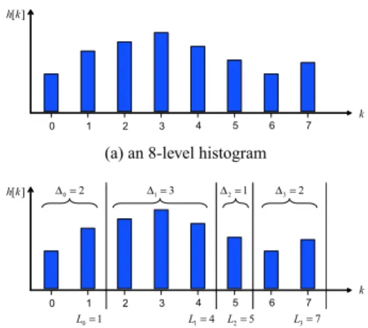
In this section, we formulate the design of a quantizer that translates a K-level discrete signal to aM-level equivalent (M <K). For this formulation, we use the histogram of the signal as the input to the quantizer. Thek-th element of the histogram ish[k] (k=0,· · ·,K−1), which is the frequency of signal valuek. For example, in the case of an 8-bit signal, the range ofkis 0 to 255. The formulated quantizer is defined using two parameters∆mandLm;∆mis the length of them-th sub-interval of the histogram. Lm is the upper boundary of them-th sub-interval in the histogram. In the following, Lmis simply called boundary. The boundaries are described as follows:









 Lm=

m

X

j=0

∆j−1 (m=0,· · ·,M−2) LM−1=K−1

(1)

Henceforth, them-th interval [Lm−(∆m−1),Lm] of the histogram is called them-th bin. Since each bin is set to have at least one element,L_m(0≤m≤M−2) is restricted in the following range:

m≤Lm≤K−(M−m) (2) Figure 1 illustrates the above-mentioned parameters for the case where the histogram with eight elements (K = 8) is quantized to one with four bins (M =4). Figure 1 (b) shows each bin contains 2(= ∆0) elements, 3(= ∆1) elements, 1(=

∆2) element, and 2(= ∆3) elements of the input histogram, respectively; and the upper boundary of each bin becomes L0 = ∆0−1=1,L1 =L0+ ∆1 =4,L2 =L1+ ∆2=5, and L3=L2+ ∆3=7, respectively.

Quantizer design is based on minimizing the quantization error created by approximating all values in the m-th bin [Lm−(∆m−1),Lm] in the histogram with representative value ˆc(∆m,L_m). As the quantization error of the m-th bin [Lm−(∆m−1),Lm], we use the summation of square error

Fig. 1 Example of parameters for quantization.

(3)

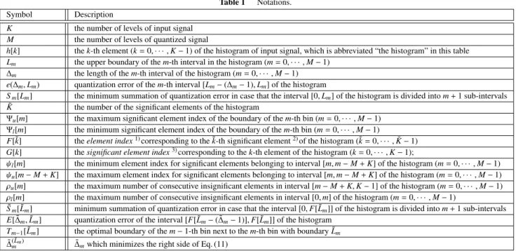
Table 1 Notations.

Symbol Description

K the number of levels of input signal M the number of levels of quantized signal

h[k] thek-th element (k=0,· · ·,K−1) of the histogram of input signal, which is abbreviated “the histogram” in this table L_m the upper boundary of them-th interval in the histogram (m=0,· · ·,M−1)

∆m the length of them-th interval of the histogram (m=0,· · ·,M−1) e(∆m,L_m) quantization error of them-th interval [Lm−(∆m−1),L_m] of the histogram

S_m[Lm] the minimum summation of quantization error in case that the interval [0,L_m] of the histogram is divided intom+1 sub-intervals K˜ the number of the significant elements of the histogram

Ψu[m] the maximum significant element index of the boundary of them-th bin (m=0,· · ·,M−1) Ψl[m] the minimum significant element index of the boundary of them-th bin (m=0,· · ·,M−1)

F[˜k] theelement index¹⁾corresponding to the ˜k-th significant element²⁾of the histogram (˜k=0,· · ·,K˜−1) G[k] thesignificant element index³⁾corresponding to thek-th element of the histogram (k=0,· · ·,K−1);

ψl[m] the minimum element index for significant elements belonging to interval [m,m−M+K] of the histogram (m=0,· · ·,M−1) ψu[m−M+K] the maximum element index for significant elements belonging to interval [m,m−M+K] of the histogram (m=0,· · ·,M−1) ρu[m] the maximum number of consecutive insignificant elements in interval [m−M+K,K−1] of the histogram (m=0,· · ·,M−1) ρl[m] the maximum number of consecutive insignificant elements in interval [0,m] of the histogram (m=0,· · ·,M−1)

S˜_m[ ˜L_m] minimum summation of quantization error in case that the interval [0,F[ ˜L_m]] of the histogram is divided intom+1 sub-intervals E[ ˜∆m,L˜_m] quantization error of the interval [F[ ˜L_m−( ˜∆m−1)],F[ ˜L_m]] of the histogram

Tm−1[ ˜Lm] the optimal boundary of them−1-th bin next to them-th bin with boundary ˜Lm

∆˜^{( ˜}m^L^m⁾ ∆˜mwhich minimizes the right side of Eq. (11)

1)Element indexis an index to identify each element of the histogram.

2)The significant elements are listed in a sequence and each significant element in the sequence is referred by index ˜k.

3)Significant element indexis an index to identify each significant element of the histogram. Note that look-up tableG[k] provides the inverse mapping of look-up tableF[˜k], and vice versa.

e(∆m,Lm) defined as follows:

e(∆m,Lm)=

L_m

X

k=L_m−∆m+1

{k−c(ˆ ∆m,Lm)}²h[k] (3) where ˆc(∆m,Lm) is the integer value that is the closest to the centroid of them-th bin [L_m−(∆m−1),L_m]. The centroid is defined as follows:

c(∆m,Lm)= PL_m

k=L_m−(∆m−1)kh[k]

PL_m

k=L_m−(∆m−1)h[k] (4) Note that each bin is set so that the denominator of equation (4) does not become zero. In other words, each bin is set so as to include at least one significant element. Optimizing the quantizer means finding the parameters that minimize the following summation of quantization error

(∆^∗0,· · · ,∆^∗M−1)=arg min

∆0,···,∆M−1











M−1

X

m=0

e(∆m,Lm)











(5) 3. DP Quantization

In this section, we describe DP quantization, the basic algorithm of our proposed method. This description of DP quantization will help to clarify the difference between DP quantization and our proposed method described in Sect. 5 and allow a better understanding of our proposed method.

In the optimization problem of Eq. (5), the number of combinations ofMparameters (∆0,· · · ,∆M−1) grows expo- nentially. Using the brute force method to search for the optimal combination, (∆^∗₀,· · ·,∆^∗_M−1), takes exponential time

and is not realistic in terms of complexity.

Considering that the quantization errore(∆m,Lm) of the m-th bin depends on the boundaryLmof them-th bin and the width∆mof the same bin, dynamic programming based approaches (DP quantization) [9]–[11] have been used to solve the optimization problem of Eq. (5).

DP quantization focuses on a recurrence relation of quantization error. We define Sm[Lm] for each Lm (m = 0,· · ·,M −1) as the minimum summation of quantization error Pm

i=0e(∆i,Li) where the interval [0,Lm] of histogram h[k] (k = 0,· · ·,K−1) is divided intom+1 bins. Since e(∆m,Lm) depends onLmand∆m,Sm[Lm] can be expressed usingS_m−1[L_m−∆m] in the following recursive equation:

Sm[Lm]=min

∆m

{Sm−1[Lm−∆m]+e(∆m,Lm)} (6) wherem=1,· · ·,M−1 andL_m=m,· · ·,K−(M−m). Using Eq. (6), the computation ofSm[Lm] results in the selection of the best parameter among the values of ∆m =1,· · ·,L_m− m+1. The range of∆mis described in Appendix A.

Applying Eq. (6) to Eq. (5), the minimization problem of Eq. (5) becomes as follows:

min∆M−1

{SM−2[LM−1−∆M−1]+e(∆M−1,LM−1)} (7) Furthermore, applying Eq. (6) recursively and noting LM−1 =K−1 in Eq. (1), the minimization problem of Eq. (5) is to find the optimal solution (∆^∗₀,· · · ,∆^∗_M−1) from among

1

2M³−^2K₂⁺⁵M²+ ^K²⁺^7K₂ ⁺⁴M−K²−K candidates^†. Thus,

†This number is derived in Appendix C as the number of candidate paths in a trellis diagram that is described in Sect. 4.

(4)

DP quantization can provide a polynomial time solution to the minimization problem.

4. Interpretation of DP Quantization as Optimal Path Search

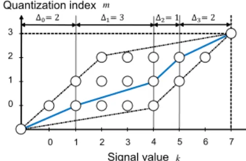
Using a trellis transition diagram, we provide an interpretation of the optimization process of DP quantization. This interpretation will be useful in understanding the proposed algorithm described in Sect. 5. The trellis transition diagram of Fig. 2 illustrates the quantization result for the example shown in Fig. 1(b). In Fig. 2, the vertical axis and the horizontal axis represent signal valuesk ∈ {0,1,· · ·,7} and quantization indicesm ∈ {0,1,2,3}, respectively. The node at (k,m) in the trellis transition diagram has a cost value that is the minimum summation of quantization error caused by approximating interval [0,k] in the histogram withm+1 levels. For example, the node at (4,1) has the minimum summation of quantization error that is generated by using two representative values to quantize the five elements (k= 0,· · · ,4) of the histogram. Note that the node on the bottom-left corner is a dummy node introduced as the start node and does not have a cost value. Each path in the trellis transition diagram has a cost that is quantization error for a histogram interval determined by both endpoints of the path.

For example, the cost of the path from node (1,0) to node (4,1) becomes the quantization error caused by quantizing the histogram interval [2,4] as the second bin. Quantiza- tion shown in Fig. 1(b) corresponds to traversed paths indicated by the bold blue line in the trellis transition diagram of Fig. 2. The horizontal displacement of each traversed path is its interval length. For example, traversed paths indicated by the bold blue line have four paths whose horizontal displacements are 2(= ∆0), 3(= ∆1), 1(= ∆2) and 2(= ∆3), respectively. Thus, the design of the optimal quantizer can be represented as the optimal path search over the trellis transition diagram.

Using the trellis transition diagram, we can interpret the reduction in complexity of optimal quantization offered by dynamic programming as follows. Let us focus on a red node in Fig. 3. The red node has four traversable paths from gray nodes. The traversable paths are characterized by horizontal displacements (1, 2, 3, and 4) corresponding to∆2. When we try to find the optimal path up to the red node in Fig. 3, it is not necessary to search all paths from the start node to the red node. It is enough to search paths from each gray node to the red node. This is because each gray node has an accumulated cost that is equal to the minimum summation of quantization error corresponding to the optimal path from the start node up to each gray node. Evaluating the summation of the accumulated cost stored in a gray node and the cost provided on the path from the gray node to the red node, we can identify the minimum summation of quantization error as corresponding to the optimal path that con- nects the start node to the red node through the gray node.

Fig. 2 Traversed path corresponding to quantization shown in Fig. 1(b).

Fig. 3 Optimal path search for red node.

5. Sparse DP Quantization

5.1 Focus for Complexity Reduction

In this section, we introduce a complexity reduction algorithm for DP quantization that focuses on insignificant elements with zero-frequency. When the signal value Lm+1 has zero-frequency, that is,h[Lm+1] =0, the quantization error of interval [Lm−(∆m−1),Lm+1] in the histogram is equal to that of interval [Lm−(∆m−1),Lm]. This is because h[L_m+1](=0) has no effect on the quantization error. Thus, in the case ofh[Lm+1]=0, we can skip the computation of S_m[L_m+1] indicated by Eq. (6). In other words, for minimization of quantization error, it is enough to consider only significant elements whose frequencies are non-zero.

In order to verify sparseness of signal values, we as- sessed standard images described later in Sect. 6. The sparseness of each color channel is defined as the ratio of the number of insignificant elements to the number of all elements, as follows:

Sparseness= the number of insignificant elements the number of all elements

(8) Table 2 confirms that all images examined have sparseness to some extent.

5.2 Restriction of Search Range Considering Sparseness Considering sparseness, it is possible to skip some elements

(5)

Table 2 Sparseness of standard images (cells in the “Sparseness” column represent values given by Eq. (8)).

Image G-channel Sparseness [%]

Image01 64.1

Image02 62.4

Image03 63.4

Image04 63.4

Image05 63.4

Image06 63.4

Image07 63.5

Image08 64.0

Image09 63.5

Image10 65.4

Image11 56.6

Image12 57.7

Image13 69.7

Image14 57.9

Image15 64.9

Image16 62.1

Image17 58.2

Image18 58.4

Image19 63.5

Image20 57.4

Image21 57.9

Image22 57.3

Image23 57.2

Image24 57.7

Image25 57.3

Image26 58.1

R-channel B-channel Sparseness [%] Sparseness [%]

64.1 62.5

62.5 62.4

63.4 63.4

63.7 63.4

63.4 63.4

63.7 66.4

64.4 63.4

63.7 65.3

65.5 67.5

57.1 56.4

56.3 59.4

69.4 67.1

57.8 56.8

65 62.7

61.3 60.4

60.9 56.8

60.6 56.4

62.1 59.4

58.2 56.6

56.5 60

59.7 56.4

56.8 56.5

58.3 56.3

59.3 56.5

56.5 56.3

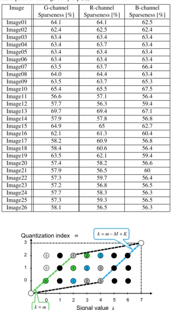
Fig. 4 Insignificant nodes (black circles) and significant nodes (circles with numeral) in the case ofK=8 andM=4.

of a histogram in DP quantization. Before explaining de- tailed algorithm, we provide its basic idea using a toy example. In preparation for description of the proposed quantization algorithm, we define some symbols and terminolo- gies below. Indexkidentifies an element of histogramh[k]

(k=0,· · ·,K−1). The index is calledelement index. ˜Krep- resents the number of significant elements of the histogram.

Those significant elements are listed in a sequence and each significant element in the sequence is referred by index ˜k (˜k=0,· · ·,K˜ −1). The index is calledsignificant element index.

Figure 4 provides an example of a trellis transition diagram whose elements withk=1,5,6 are insignificant for the case of M = 4 and K = 8. The nodes in the trellis transition diagram are classified into two types, significant node and insignificant node. Significant node is located in

the position where the abscissa is a significant element. In- significant node is located in the position where the abscissa is an insignificant element. In this figure, significant nodes and insignificant nodes are represented by circles with numeral and black circles, respectively. The numeral in each circle represents the significant element index.

As described in Sect. 2, the boundary of each bin is in the range defined by inequality (2). In Fig. 4, the blue broken line and the green broken line correspond to superior end and inferior end defined by inequality (2). Thus, the optimal path is restricted to candidates that pass through nodes located between the green broken line and the blue broken line.

If there are any insignificant elements in a quantized histogram, insignificant elements can be excluded from the candidates for the boundary of each bin. From the viewpoint of searching the optimal path in the trellis transition diagram, it is not necessary to search paths via insignificant nodes. Thus, the search range for the optimal path is restricted to candidates that pass through significant nodes within a parallelogram area surrounded by broken-lines.

Furthermore, the leftmost nodes within the search range can be additionally restricted according to the source nodes of the transition. Let us consider the leftmost node within the search range in each row in the trellis transition diagram. In the followings, the node located at the position ofk=κandm=µis referred as “node (κ,µ)”. In the case of the 0-th row (m=0), the node (0,0) on the green broken line is a significant node. This node is identified as the leftmost node in this row. In the case of the first row (m=1), the node (1,1) on the green broken line is an insignificant node. In the right side of the green broken line, the closest significant node to the node (1,1) is node (2,1) indicated by a green circle with the numeral of one. In the case of the second row (m=2), although node (2,2) on the green broken line is a significant node, this node is excluded from candidates for searching the optimal path. This is because the transition source to the node (2,2) is only node (1,1), which is excluded from candidates for searching the optimal path as stated in the case ofm=1. Thus, as the leftmost node in this row, node (3,2) is identified.

Similarly, the rightmost nodes within the search range can be additionally restricted according to the destination nodes of the transition. Let us consider the rightmost node within the search range in each row. In the case ofm =1, node (5,1) on the blue broken line is an insignificant node.

In the left side of the blue broken line, the closest significant node to the node (5,1) is node (4,1). But, this node is excluded from candidates for searching the optimal path as well as insignificant nodes. This is because there are no possible paths to transit from the node (4,1). The destination to transit from the node (4,1) is only node (5,2) and (6,2), which are insignificant nodes. Thus, as the rightmost node in this row, we select node (3,1) indicated by a blue circle with the numeral of two. In the case ofm=0, as with the case ofm =1, although node (4,0) on the blue broken line and node (3,0) are significant nodes, these nodes are

(6)

excluded from candidates for searching the optimal path.

This is because there are no possible paths to transit from the node (4,0) and (3,0). The destination to transit from the node (4,0) is only node (5,1) which is an insignificant node, and those from the node (3,0) are node (5,1) and (4,1) which are excluded from candidates for searching the optimal path as stated in the case ofm=1. Thus, as the rightmost node in this row, we select node (2,0) indicated by a blue circle with the numeral of one.

The above-illustrated restriction of the nodes in the trellis diagram are formulated as the range specification of the index of each bin. The leftmost node within the search range in them-th row is identified as the minimum significant element index of the boundary ofm-th bin, which is referred as the lower limit of them-th bin, hereinafter. For the lower limit of them-th bin, tableΨl[m] (m=0,· · ·,M−1) is prepared.Ψl[m] (m=0,· · · ,M−1) is generated as follows:

Ψl[m]=











G[max(ψl[m],m+ρl[m])]

(m=0,· · · ,M−2) K˜ −1 (m=M−1)

(9)

where, tableG[k] lists the significant element index corresponding to thek-th element. max() returns the greater of the given values. ψ_l[m] is the minimum element index for significant elements belonging to interval [m,m−M+K].

In the example of Fig. 4,ψ_l[m] indicates the closest significant node to the green broken line in the right side of the green broken line. In other words,ψ_l[m] indicates the significant element which is the closest to the inferior end in the range for the boundaryLmof them-th bin. ρ_l[m] is the maximum number of consecutive insignificant elements in interval [0,m], and is generated according to the process shown in Fig. 5. In the example of Fig. 4, the element indexm+ρl[m] in the above equation can be interpreted as follows. ρ_l[m] is the maximum number of consecutive insignificant elements in the left side of the green broken line and on itself, that is,ρ_l[0] =0,ρ_l[1]=ρ_l[2]=1. mcorre- sponds to the element index of the node on the green broken line. Thus, the element indexm+ρ_l[m] indicates the leftmost node among candidates whose transition source are limited to significant nodes.

The rightmost node within the search range in them-th row is identified as the maximum significant element index of the boundary ofm-th bin, which is referred as the upper limit of them-th bin, hereinafter. For the upper limit of the m-th bin, tableΨu[m] (m=0,· · ·,M−1) is prepared.Ψu[m]

(m=0,· · ·,M−1) is generated as follows:

Ψu[m]=G[min(ψu[m−M+K], m−M+K−ρu[m])]

(m=0,· · ·,M−1)

(10)

where min() returns the smaller of the given values.ψ_u[m− M+K] is the maximum element index for significant elements belonging to interval [m,m−M+K] of the histogram.

1. ifh[0],0

2. c←0

3. ρl[0]←0 4. else

5. c←1

6. ρl[0]←1 7. form=1,· · ·,M−1 8. ifh[m],0

9. c←0

10. else

11. c+ +

12. ρl[m]←max(ρl[m−1],c)

Fig. 5 Generation algorithm for look-up-tableρl[m].

1. ifh[K−1],0

2. c←0

3. ρu[M−1]←0 4. else

5. c←1

6. ρu[M−1]←1 7. form=M−2,· · ·,0 8. ifh[m−M+K],0

9. c←0

10. else

11. c+ +

12. ρu[m]←max(ρu[m+1],c)

Fig. 6 Generation algorithm for look-up-tableρu[m].

In the example of Fig. 4,ψ_u[m−M+K] corresponds to the closest significant node to the blue broken line in the left side of the blue broken line. In other words,ψ_u[m−M+K]

indicates the significant element which is the closest to the superior end in the range for the boundary Lm of them-th bin.ρu[m] is the maximum number of consecutive insignificant elements in interval [m−M+K,K−1], and is generated according to the process shown in Fig. 6. In the example of Fig. 4, the element indexm−M+K−ρu[m] in the above equation can be interpreted as follows. ρ_u[m] is the maximum number of consecutive insignificant elements in the right side of the blue broken line and on itself, that is, ρu[0] = ρu[1] =2, ρu[2] =1. m−M+Kcorresponds to the element index of the node on the blue broken line. Thus, the element index m−M +K−ρu[m] indicates the rightmost node among candidates whose transition destinations are limited to significant nodes.

5.3 Optimal Quantizer Design Considering Sparseness In this subsection, we describe our algorithm of sparse DP quantization that reduces the complexity by skipping computation for insignificant elements while retaining optimality in terms of minimizing quantization error. In the following, we use tableF[˜k] that lists the element index corresponding to the ˜k-th significant element.

Let us consider dividing histogram interval [0,F[ ˜Lm]], whose boundary is the ˜Lm-th significant element, intom+1 bins. The sub-interval [F[ ˜Li − ( ˜∆i −1)],F[ ˜Li]] (where,

(7)

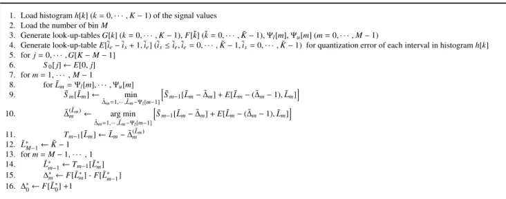
1. Load histogramh[k] (k=0,· · ·,K−1) of the signal values 2. Load the number of binM

3. Generate look-up-tablesG[k] (k=0,· · ·,K−1),F[˜k] (˜k=0,· · ·,K˜−1),Ψl[m],Ψu[m] (m=0,· · ·,M−1)

4. Generate look-up-tableE[˜i_e−˜i_s+1,˜i_e] (˜i_s≤˜i_e,i˜_e=0,· · ·,K˜−1,i˜_s=0,· · ·,K˜−1) for quantization error of each interval in histogramh[k]

5. forj=0,· · ·,G[K−M−1]

6. S₀[j]←E[0,j]

7. form=1,· · ·,M−1

8. for ˜L_m= Ψl[m],· · ·,Ψu[m]

9. S˜m[ ˜Lm]← min

∆˜m=1,···,L˜_m−Ψl[m−1]

hS˜m−1[ ˜Lm−∆˜m]+E[ ˜Lm−( ˜∆m−1),L˜m]i

10. ∆˜^{( ˜}m^L^m⁾← arg min

∆˜m=1,···,˜Lm−Ψl[m−1]

hS˜_m−1[ ˜L_m−∆˜m]+E[ ˜L_m−( ˜∆m−1),L˜_m]i

11. T_m−1[ ˜L_m]←L˜_m−∆˜^{( ˜}m^L^m⁾

12. ˜L^∗_M−1←K˜−1 13. form=M−1,· · ·, 1 14. L˜^∗

m−1←T_m−1[ ˜L^∗_m] 15. ∆^∗m←F[ ˜L^∗_m] -F[ ˜L^∗

m−1] 16. ∆^∗0←F[ ˜L^∗₀]+1

Fig. 7 Sparse DP quantization algorithm.

i=0,· · ·,m) of the interval [0,F[ ˜L_m]] is thei-th bin. ˜∆iis the number of significant elements in thei-th bin, and ˜Liis the significant element index of the boundary of thei-th bin, in other words, ˜Liis the maximum significant index among significant elements in thei-th bin. We compute quantization errore(F[ ˜Li]−F[ ˜Li−( ˜∆i−1)]+1,F[ ˜Li]) caused by using the centroid value to approximate all values in thei-th bin. This error is stored in look-up table E[ ˜∆i,L˜i] and re- fer to the entries as needed, in order to eliminate duplicate computations for quantization error. We define a look-up table to store the minimum summation of quantization er- rorPm

i=0E[ ˜∆i,L˜_i] as ˜S_m[ ˜L_m]. Note that ˜S_m[ ˜L_m] is equal to Sm[F[ ˜Lm]].

SinceE[ ˜∆m,L˜_m] depends on the significant element index ˜Lmof the boundary of them-th bin and the number of significant elements ˜∆min them-th bin, the value stored in S˜m[ ˜Lm] is computed using ˜Sm−1[ ˜Lm−∆˜m] as follows:

S˜m[ ˜Lm]=min

∆˜m

nS˜m−1[ ˜Lm−∆˜m]+E[ ˜∆m,L˜m]o

(11) wherem=1,· · ·,M−1. Using recursive equation (11), the computation of ˜Sm[ ˜Lm] results in the selection of the optimal parameter ˜∆mamong 1,· · ·,L˜_m−Ψl[m−1]. The range of

∆˜mcan be found in Appendix B. Considering that the upper limit and the lower limit of significant indices in them-th bin are defined asΨu[m] andΨl[m] respectively, ˜Lmcan be taken from Ψl[m] to Ψu[m]. The value stored in ˜Sm[ ˜Lm] is used in computing ˜Sm+1[ ˜Lm+1]. In the case of m = 0, S˜0[ ˜L0] represents the quantization error caused by using the centroid to approximate histogram interval [0,F[ ˜L0]], and we obtain:

S˜0[ ˜L0]=E[0,F[ ˜L0]]

The optimal boundary of them−1-th bin, which is next to them-th bin with boundary ˜Lm(= Ψl[m],· · ·,Ψu[m]), is stored in tableTm−1[ ˜L_m] as follows:

Tm−1[ ˜Lm]=L˜m−∆˜^{( ˜}m^L^m⁾

where ˜∆^{( ˜}m^L^m⁾ denote ˜∆m which minimizes the right side of Eq. (11). Casting the above processes in pseudo-code yields instructions 4 to 11 in Fig. 7. Instruction 3 in Fig. 7 generates the look-up tables Ψl[], Ψu[] described in Sect. 5.2 andG[],F[]. Instruction 4 generates a look-up-table that stores the quantization error of every interval in the histogram. The stored value inE[˜ie−˜is+1,˜ie] (˜is ≤ ˜ie,˜ie = 0,· · ·,K˜−1,˜is=0,· · · ,K˜ −1) is the quantization error of the interval [F[˜is],F[˜ie]] in the histogram. ˜isand ˜ieare significant element indices that identify an interval in the histogram. The minimization problem of Eq. (5) is rewritten as the following recursive formulation:

min˜

∆M−1

nS˜M−2[ ˜LM−1−∆˜M−1]+E[ ˜∆M−1,L˜M−1]o

In the final step at the instruction 10 in Fig. 7, we obtain

∆˜^{( ˜}_M−1^L^M−1⁾as follows:

∆˜^{( ˜}_M−1^L^M−1⁾ =arg min

∆˜M−1

nS˜M−2[ ˜LM−1−∆˜M−1]+E[ ˜∆M−1,L˜M−1]o

The optimal parameters (∆^∗₀,· · · ,∆^∗_M−1) are obtained from the following process, the back-track process. Since the possible value of ˜LM−1 is limited to ˜K−1, as the optimal value of ˜LM−1, we have ˜L^∗_M−1 = K˜ −1. By using ˜L^∗_M−1 = K˜ −1 and referring to table T_M−2[], we obtain ˜L^∗_M−2 = TM−2[ ˜L^∗_M−1]. Similarly, we obtain ˜L^∗_M−3 = TM−3[ ˜L^∗_M−2] ,· · ·, ˜L^∗₀=T0[ ˜L^∗₁] as the significant element indices of the boundary of each bin. By accessingF[] with these obtained significant element indices ˜L^∗_M−1, ˜L^∗_M−2,· · ·, L˜^∗₀, we get the element indices of the boundary of each bin.

As a result, the intervals of each bin are derived as follows:

∆^∗_M−1 = F[ ˜L^∗_M−1]−F[ ˜L^∗_M−2],∆^∗_M−2 = F[ ˜L^∗_M−2]−F[ ˜L^∗_M−3] ,· · ·,∆^∗₁ =F[ ˜L^∗₁]−F[ ˜L₀^∗],∆^∗₀=F[ ˜L^∗₀]+1. Casting the above- mentioned processes in pseudo-code yields instructions 12 to 16 in Fig. 7.

(8)

6. Experiments

We performed the following experiments in order to in- vestigate the effectiveness of our quantization algorithm from the viewpoint of complexity. As the input signal of each quantization algorithm, we used the sequences in ITE/ARIB Ultra-high definition/wide-color-gamut standard test sequences - Series A, Series B [19], [20]^†. The sequences employ the progressive scan format with resolu- tion of 3840×2160 pixels/frame in the RGB4:4:4 color format defined as ITU-R Recommendation BT.2020. The sequences are provided as still serial number files in uncom- pressed DPX format[21]. Pixel values of RGB components in the DPX file are treated as 16-bit integers. Since the actual pixel value only has 12 bit depth, it is stored in the higher 12 bits of the 16-bit integer and the remaining 4 bits are set to 0. In other words, these signals were sampled at 12 bit scale, soK =4096. By extracting the higher 12 bits of each color component for every pixel, we obtained the evaluation data. Each color channel signals of the 61th frame^††

of each sequence were used in the following evaluation experiments. Given the existence of legacy displays, it is often necessary to convert high bit depth signals into low bit depth signals that have just ten or eight bits/channel. Accordingly, we setM =1024,256 as the number of bins. Additionally, we also investigated the cases of M = 512,128 for considering the characteristic of the proposed algorithm due to change in the number of bins. These experiments were performed on a computer with CPU:Intel core i7 (2.8 GHz) and memory: 8 GB.

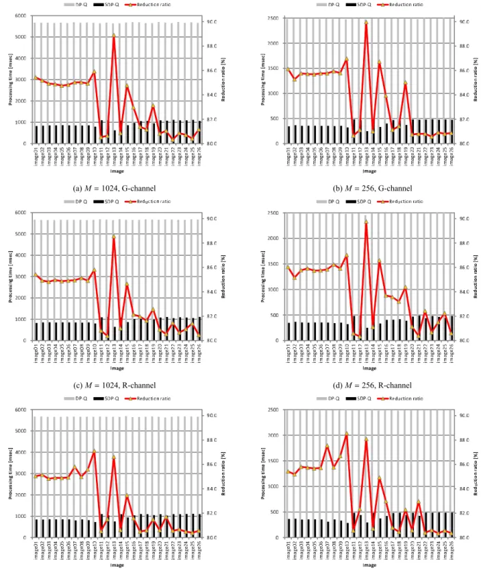
In order to evaluate the complexity reduction achieved by sparse DP quantization, we compared sparse DP quantization (abbreviated to SDP-Q) with DP quantization (abbreviated to DP-Q) described in Sect. 3, in terms of processing time. The results are shown as bar graphs in Fig. 8, where processing time is the average of 100 trials. Additionally, we evaluated the complexity reduction attained by SDP-Q using the following metric:

complexity reduction ratio=

processing time of DP-Q−processing time of SDP-Q

processing time of DP-Q (12)

The line graphs in Fig. 8 show the complexity reduction ratio for each image. From Table 2 and Fig. 8, we can confirm that the complexity reduction ratio improves as sparseness increases. In order to elucidate the overall performance for all images, Table 3 shows average DP-Q and SDP-Q processing times for all images at every M value. From this table, we can confirm that sparse DP quantization can, rela- tive to DP quantization, reduce complexity by 82.9 to 84.2%

on average. Additionally, Table 4 shows the breakdown of

†Only Japanese manuals are available now. The Web site of the ITE says that English version is being made at present.

††The 61th frame is the head frame that contains captured scenes. The first 60 frames capture caption telop only.

the processing time of SDP-Q; look-up table (LUT) generation processes corresponding to instruction 3 and 4 in Fig. 7, and search processes corresponding to the other instructions in Fig. 7. It is observed that “search processes” has strong effect in the total processing time.

In order to evaluate computing time reduced by SDP- Q with differentMvalues, we applied analysis of variance (ANOVA) to complexity reduction ratio with M. Table 5 shows the results of ANOVA test for complexity reduction ratio. In this case, the critical value at the 5% significance level is found 2.6955 from the F-distribution table. It was observed that F-ratio values for every color channel in Ta- ble 5 were less than the critical value. Thus, we could not reject the null hypothesis that four kinds of M values produce the same expected values of complexity reduction ratio. That is, we could not obtain statistical evidence that there was significant difference among the expected values of complexity reduction ratio with four kinds ofMvalues.

Next, we analyze the complexity of the search processes and the LUT generation processes. The search processes conduct the following P1. As a dominant factor in the generation of look-up tables, let us focus on that of look-up tableE[] which conducts the following P2.

(P1) optimal path search based on DP recursive equation (P2) construction of look-up tableE[] to store quantization

error for each quantized bin

The complexity of “P1” is related to the number of fea- sible paths within the search range. In the following, feasi- ble path within the search range is abbreviated to candidate path. The number of candidate paths for DP-Q is derived fromKandMas follows:

Ωpath(M,K)

= 1

2M³−2K+5

2 M²+K²+7K+4

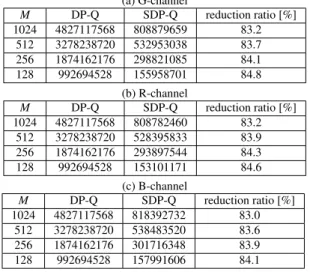
2 M−K²−K (13) The derivation of the above equation can be found in Ap- pendix C. The figures in column “DP-Q” in Table 6 were generated based on the above equation. By contrast, the number of candidate paths for SDP-Q could not be derived like DP-Q due to the restriction of search range described in Sect. 5.2. So, we counted up candidate paths for each image for everyM, and computed the average number of all images for everyMvalue. These average numbers are shown as the figures in column “SDP-Q” in Table 6. The figures in column “reduction ratio” in Table 6 are computed by applying the same concept as Eq. (12) to the candidate paths of DP- Q and SDP-Q. We evaluated the number of candidate paths reduced by SDP-Q through applying ANOVA to its reduction ratio with differentMvalues. Table 7 shows the results of the above-mentioned ANOVA test. It was observed that F-ratio values for every color channel in Table 7 were less than the critical value (2.6955) at the 5% significance level.

Thus, we could not reject the null hypothesis that four kinds ofMvalues produce the same expected values of the above- mentioned reduction ratio.

(9)

Fig. 8 Processing time of DP-Q and SDP-Q (bar graphs labeled “DP-Q” are processing times for DP quantization, bar graphs labeled “SDP-Q” are processing times for SDP quantization, and “Reduction ratio” are values defined in Eq. (12)).

The complexity of “P2” is related to the number of intervals in the input histogram. In the following, the quantized bin is abbreviated to candidate interval. The number of candidate intervals for DP-Q is derived fromKandMas

follows:

Ωinterval(M,K)=(−M²+M+K²+K)/2 (14) The derivation of the above equation can be found in Ap-

(10)

Table 3 Average processing time of DP-Q and SDP-Q of all images in everyM(cells in the “Reduction ratio” column represent values defined in Eq. (12)).

(a) G-channel

M DP-Q SDP-Q reduction ratio

[msec] [msec] [%]

1024 5667.5 957.6 83.1

512 4000.0 662.6 83.4

256 2490.0 406.8 83.7

128 1546.1 248.2 83.9

(b) R-channel

[msec] [msec] [%]

1024 5666.0 957.0 83.1

512 3996.2 657.9 83.5

256 2488.8 400.5 83.9

128 1546.6 244.1 84.2

(c) B-channel

[msec] [msec] [%]

1024 5665.7 969.3 82.9

512 4001.3 670.2 83.2

256 2491.6 410.9 83.5

128 1548.7 252.1 83.7

Table 4 The breakdown of processing time of SDPQ (“LUT generation processes consist of instruction 3 and 4 in Fig. 7, and “search processes”

consist of the other instructions in Fig. 7).

(a) G-channel

M LUT generation processes search processes

1024 43.6 914.1

512 71.5 591.1

256 77.4 329.4

128 77.8 170.4

(b) R-channel

1024 42.3 914.7

512 70.4 587.5

256 76.0 324.5

128 76.8 167.3

(c) B-channel

1024 46.0 923.3

512 73.5 596.7

256 79.5 331.4

128 79.8 172.3

pendix D. The figures in column “DP-Q” in Table 8 were generated based on the above equation. By contrast, candidate intervals for SDP-Q were counted for each image for every M. The average number of candidate intervals for everyM value was computed. These average numbers are shown as the figures in column “SDP-Q” in Table 8.

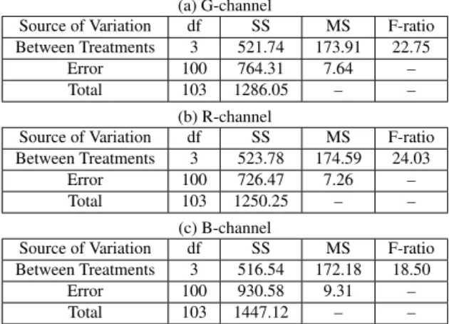
We evaluated the number of candidate intervals reduced by SDP-Q through applying ANOVA to its reduction ratio with differentM values. Table 9 shows the results of the above-mentioned ANOVA test. It was observed that F- ratio values for every color channel in Table 9 exceed the critical value (2.6955) at the 5% significance level. Thus, the ANOVA test suggested that there was significant differ- ences among the expected values of the above-mentioned

Table 5 ANOVA test results for complexity reduction ratio of processing time (df, SS and MS mean Degrees of Freedom, Sums of Squares, Mean Squares, respectively).

(a) G-channel

Source of Variation df SS MS F-ratio Between Treatments 3 10.14 3.38 0.48

Error 100 700.39 7.00 –

Total 103 710.53 – –

(b) R-channel

Error 100 625.55 6.26 –

Total 103 643.50 – –

(c) B-channel

Error 100 726.58 7.27 –

Total 103 736.59 – –

Table 6 Average number of candidate paths in everyM.

(a) G-channel

M DP-Q SDP-Q reduction ratio [%]

1024 4827117568 808879659 83.2

512 3278238720 532953038 83.7

256 1874162176 298821085 84.1

128 992694528 155958701 84.8

(b) R-channel

1024 4827117568 808782460 83.2

512 3278238720 528395833 83.9

256 1874162176 293897544 84.3

128 992694528 153101171 84.6

(c) B-channel

1024 4827117568 818392732 83.0

512 3278238720 538483520 83.6

256 1874162176 301716348 83.9

128 992694528 157991606 84.1

Table 7 ANOVA test results for reduction ratio of the number of candidate paths (df, SS and MS mean Degrees of Freedom, Sums of Squares, Mean Squares, respectively).

(a) G-channel

Error 100 696.01 6.96 –

Total 103 711.98 – –

(b) R-channel

Error 100 628.40 6.28 –

Total 103 654.88 – –

(c) B-channel

Error 100 702.54 7.03 –

Total 103 718.73 – –

reduction ratio with four kinds ofMvalues.

Let us consider how Mvalue affects the reduction ratio of the number of candidate intervals. Although we cannot derive the number of candidate intervals for SDP-