Evaluating the Asian international input-output table in comparison with the three major multiregional input-output tables

Evaluating the Asian international

input‑output table in comparison with the

three major multiregional input‑output tables

著者 Uchida Yoko, Oyamada Kazuhiko

権利 Copyrights 日本貿易振興機構（ジェトロ）アジア

経済研究所 / Institute of Developing

Economies, Japan External Trade Organization (IDE‑JETRO) http://www.ide.go.jp

journal or

publication title

IDE Discussion Paper

volume 663

year 2017‑03

URL http://hdl.handle.net/2344/00048867

INSTITUTE OF DEVELOPING ECONOMIES

IDE Discussion Papers are preliminary materials circulated to stimulate discussions and critical comments

Keywords: Multiregional Input-Output, Fragmentation, Trade in Value Added measure JEL classification: C67, F00

*Institute of Developing Economies, Japan External Trade Organization (IDE-JETRO), 3-2-2 Wakaba, Mihama-Ku, Chiba-Shi, Chiba 261-8545, Japan (yoko_uchida @ide.go.jp).

**IDE-JETRO (kazuhiko_oyamada@ide.go.jp).

IDE DISCUSSION PAPER No. 663

Evaluating the Asian International Input-Output Table

in comparison with the Three Major Multiregional Input-Output Tables

Yoko UCHIDA*, Kazuhiko OYAMADA **

March 2017

Abstract

This paper introduces the existing multiregional Input-Output (MRIO) Tables i.e., IDE, ADB, OECD, and GTAP with special attention to the method of constructing import matrix.

Also, the similarities and differences among the four MRIO Tables are studied in this paper, setting the IDE table as the benchmark. From the results of comparison of major economic indicators with WDI, IDE and OECD shows similarity to WDI, compared to GTAP and ADB. However, TiVA indicators show considerably different values in motor vehicles and motorcycles in Indonesia. Whereas there is some possibilities Indonesia’s TiVA is overestimation, it can be said that the IDE table might captures the proper production structure. In order to understand the reason why different value in the IDE table occurs, an additional survey on import demand might be required.

The Institute of Developing Economies (IDE) is a semigovernmental, nonpartisan, nonprofit research institute, founded in 1958. The Institute merged with the Japan External Trade Organization (JETRO) on July 1, 1998.

The Institute conducts basic and comprehensive studies on economic and related affairs in all developing countries and regions, including Asia, the Middle East, Africa, Latin America, Oceania, and Eastern Europe.

The views expressed in this publication are those of the author(s). Publication does not imply endorsement by the Institute of Developing Economies of any of the views expressed within.

INSTITUTE OF DEVELOPING ECONOMIES (IDE), JETRO 3-2-2, WAKABA,MIHAMA-KU,CHIBA-SHI

CHIBA 261-8545, JAPAN

©2017 by Institute of Developing Economies, JETRO

No part of this publication may be reproduced without the prior permission of the IDE-JETRO.

0

Evaluating the Asian International Input-Output Table

in comparison with the Three Major Multiregional Input-Output Tables

Yoko UCHIDA^* Kazuhiko OYAMADA^†

March 30, 2017

Abstract

This paper introduces the existing multiregional Input-Output (MRIO) Tables i.e., IDE, ADB, OECD, and GTAP with special attention to the method of constructing import matrix.

Also, the similarities and differences among the four MRIO Tables are studied in this paper, setting the IDE table as the benchmark. From the results of comparison of major economic indicators with WDI, IDE and OECD shows similarity to WDI, compared to GTAP and ADB. However, TiVA indicators show considerably different values in motor vehicles and motorcycles in Indonesia. Whereas there is some possibilities Indonesia’s TiVA is overestimation, it can be said that the IDE table might captures the proper production structure. In order to understand the reason why different value in the IDE table occurs, an additional survey on import demand might be required.

Keywords: Multiregional Input-Output, Fragmentation, Trade in Value Added measure JEL Classification Numbers: C67, F00

* Institute of Developing Economies, Japan External Trade Organization (IDE-JETRO), 3-2-2 Wakaba, Mihama-Ku, Chiba-Shi, Chiba 261-8545, Japan (yoko_uchida @ide.go.jp).

† IDE-JETRO (kazuhiko_oyamada@ide.go.jp).

1

1. Introduction

Importance of intermediate input trade and production fragmentation has been focused in explaining the growth in world trade in recent years. Manufacturing goods are no longer produced in a single country. Production processes are subdivided into several stages, in which respective countries specialize according to their own comparative advantages.

Many countries are involved in production fragmentation in order to produce just single final goods to consumers (Uchida and Inomata, 2008). Existing trade statistics framework cannot trace out such production fragmentation, since it cannot specify intermediate and final goods transactions within and between countries at industry/commodity sector level (Koopman, Wang and Wei, 2014). The data in need by researchers is the value of import transaction of each commodity by source, destination and agents, i.e., producer, consumer and government. Multiregional Input-Output (MRIO) table is useful data to capture current situation of production sharing in that it contains detailed information on import-sourcing by industry/commodity and distinction between different uses whether commodities are for final consumption or intermediate consumption.

Institute of Developing Economies (IDE), Japan External Trade Organization (JETRO) compiles the foremost MRIO table beginning in 1975 and provides 6 MRIO tables thus far. The latest one is the 2005 table and it includes 10 countries, covering 76 sectors. IDE table covers broad sectors, but coverage of countries is not enough to see global production fragmentation.

Global Trade Analysis Project (GTAP) publishes 8 databases, beginning in 1990 and extending every 2 to 4 years. Each version of the database covers 57 sectors, but consists of different number of countries. The latest version of the database (GTAP version 9) covers 140 countries and reference years are 2004, 2007, and 2011 (Aguir, Narayanan, and McDougall, 2016). Unlike the MRIO tables published by other institutes, the GTAP data does not include MRIO detail, that is, import-sourcing detail. The trade flows in input-output tables in GTAP is aggregated at the border (Walmsley, Hertel and Hummels, 2016). The GTAP data has been utilized for constructing MRIO tables since it offers broad coverage of countries and sectors. Researchers have compiled their own data by utilizing the GTAP data and trade statistics in order to use the data for their own analyses. For example, Koopman, Powers, Wang, and Wei (2010) and Koopman, et al. (2014) construct the MRIO table in order to decompose gross exports into its various components by integrating the GTAP version 7 and additional trade statistics. Trefler and Zhu (2010) construct the MRIO table by utilizing GTAP version 5 and empirically assess Vanek

2

prediction¹. However, it is not a simple task for individual researchers to compile the MRIO tables, since it requires enormous amount of data and statistical work. In order to respond wide-range needs of researchers, some projects of compiling the MRIO tables have started in the late 2000’s in Europe.

The World Input-Output Database (WIOD) provides annual MRIO tables from 1995 to 2011 which consists of 40 countries and 35 sectors. The data is compiled by 12 research institutes headed by the University of Groningen, the Netherlands. Since there are only 6 countries from Asian region in WIOD, Asian Development Bank (ADB) enlarges WIOD so as to include 5 additional countries, i.e., Bangladesh, Malaysia, the Philippines, Thailand and Viet Nam. The reference year of the ADB tables are 2000, 2005-2008, and 2011 under same sector classification²as WIOD.

Organisation for Economic Co-operation and Development (OECD) provides 2015 edition of MRIO tables which includes 7 MRIO tables beginning in 1995 and extending to 2011. The data consists of 61 countries, covering 34 sectors. The Input-output tables or SUTs are obtained from national statistical office and trade data is from UN COMTRADE in order to compile the MRIO tables. Trade in value added (TiVA) indicators, which capture value added content of gross exports, are known as a useful tool to understand global value chain in recent years. OECD publishes TiVA, utilizing its MRIO tables (OECD, 2012).

EORA database provides time series MRIO tables from 1990 to 2012 which covers 189 countries and 26 sectors (Lenzen, Moran, Kanemoto, and Geschke, 2013). The data is compiled by the University of Sydney, Australia. Whereas EORA-MRIO covers the least sectors, it includes the longest time series coverage among the existing MRIO tables.

EXIOPOL (A New Environmental Accounting Framework Using Externality Data and Input-Output Tools for Policy Analysis) is an integrated project funded by the European Commission under the 6th framework program. There are two MRIO tables whose reference years are 2000 and 2007 respectively. The data covers 43 countries and 129 sectors.

Each MRIO table has proved to be useful data to depict international production fragmentation/value chain. As described above, applications of the GTAP data and OECD tables are already introduced. Baldwin and Lopez-Gonzalez (2015) pictures global pattern

1 Other examples of GTAP base MRIO are Johnson and Noguera (2012) and Andrew and Peters (2013).

2 ADB Multi-Region Input-Output Database: Sources and Methods by Mariasingham, J.

< http://www.wiod.org/otherdata/ADB/ADB_MRIO_SM.pdf>

3

of supply chain trade using the WIOD and OECD tables, showing international supply chain is mostly regional, not global. Timmer et al. (2014) measures foreign value added content using the WIOD tables and shows that the process of international fragmentation has rapidly increased since 1995. Schworer (2013) uses the WIOD tables as panel dataset and discuss the effects of offshoring on labor demand.

The question arises: how much of the similarities and differences are there among the MRIO tables? Jones, Wang, Xin, and Degain (2014) compares three major MRIO tables, i.e., GTAP, OECD, and WIOD with official statistics as well as respective results for TiVA indicators. They point out that discussing the reasons for deviation is challenging since they may originate from various aspects.

This paper is another attempt to study the similarities and differences among the four MRIO tables, i.e., IDE, ADB, OECD, and GTAP tables whose target years are 2005 for IDE, ADB, and OECD and 2004 for GTAP. Note that the ADB table instead of the WIOD table is employed in this paper, since 3 more Asian countries can be treated by employing the ADB table than by WIOD table.

The remainder of this paper is organized as follows. Section 2 illustrates feature of each MRIO tables with special attention to the method of compiling MRIO detail. In section 3, the four MRIO tables are compared with respect to selected economic indices based on the percentage deviations from the benchmark data. Sections 4 presents the discrepancies between the four MRIO tables utilizing the "mean absolute percentage difference (MAPD). Section 5 compares the based on the trade in value-added (TiVA) indicators estimated with the four MRIO data. Finally, section 6 concludes this study.

2. Features of the Four MRIO Tables

In this section, we introduce four MRIOs, i.e., IDE, ADB, OECD, and GTAP tables, with special attention to the method of constructing import-sourcing detail.

2.1. IDE Tables

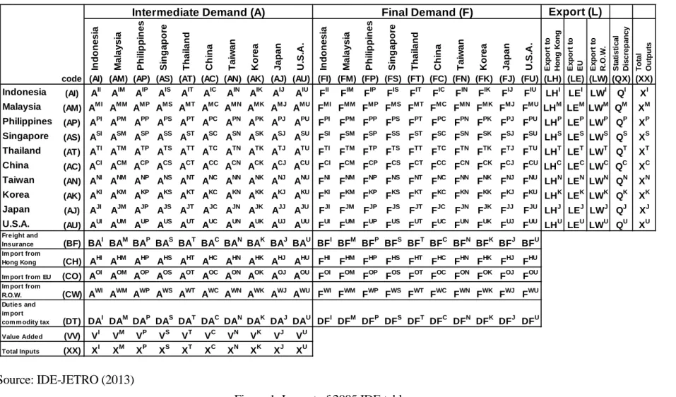
IDE-JETRO compiles the MRIO tables beginning in 1975 and provides the 6 MRIO tables thus far. The target years of the tables are 1975, 1985, 1990, 1995, 2000 and 2005. The latest table, 2005, includes 10 countries, covering 76 sectors (IDE, 2013). The layout of 2005 IDE table is shown in figure 1. The table can be read in the same manner as a national

4

input-output table. The demand side information is shown in columns, and the supply-side information in rows. Each “cell” in the table shows the input compositions of the industries of respective countries. A^II in figure 1, for instance, shows input composition of Indonesia vis-à-vis domestically produced goods and services. Also, A^MI shows imported input compositions form Malaysia to Indonesia. The cells, A^PI, A^SI, A^TI, A^CI, A^NI, A^KI, A^JI and A^UI allow the same interpretation for the imports from other countries. Final demand of Indonesia to domestically produce goods is shown in F^II. In contrast, F^MI is final demand of Indonesia for the imported goods from Malaysia. The rest of the cell can be read column-wise in the same manner as input composition. The transaction value of A^sr and F^sr (r ≠s; r, s = I, M, P, S, T, C, N, K, J, U) are valued at producer’s price of the countries of origin. A^sr and F^sr (r ≠ s; r, s = H, G, O, W) are valued at “Cost, Insurance and Freight”

(C.I.F.). International freight and insurance paid by Indonesian industries for these imported transactions are all recorded in vector BA^I. Import duties and import commodity taxes levied on all Indonesian imports are recorded in the row vector DA^I. The values in the IDE table are expressed in thousands of US dollars and exchange rate of period average from International Monetary Fund is applied for currency conversion.

The procedure of compilation of the IDE table is as follows (IDE (2006) and Kuwamori, 2016):

(a) Setting industrial sector concordance

(b) Preparing national input-output tables of the same reference year, - Conceptual adjustment

- Extension of each tables if benchmark year is not the same as other tables (c) Compiling the trade matrix by country

- Making export vector - Making import matrix - Surveys on import demand

(d) Collecting and estimating related data, i.e., transportation of costs and trade margins (TTMs), duties and import commodity taxes rate, etc.

(f) Harmonizing sectors into unified sectors

(g) Linking each national input-output table via trade flows (h) Reconciliation of the data

National input-output tables are obtained from national statistical office or collaborating institutes if the data from national statistical office is not available. Almost all of the MRIO tables are constructed under same procedure, but compilation method of import matrix makes difference of each table.

5 Source: IDE-JETRO (2013)

Figure 1: Layout of 2005 IDE table

Indonesia Malaysia Philippines Singapore Thailand China Taiwan Korea Japan U.S.A. Indonesia Malaysia Philippines Singapore Thailand China Taiwan Korea Japan U.S.A. Export to Hong Kong Export to EU Export to R.O.W. Statistical Discrepancy Total Outputs

code (AI) (AM) (AP) (AS) (AT) (AC) (AN) (AK) (AJ) (AU) (FI) (FM) (FP) (FS) (FT) (FC) (FN) (FK) (FJ) (FU) (LH) (LE) (LW) (QX) (XX) Indonesia _(AI) A^II A^IM A^IP A^IS A^IT A^IC A^IN A^IK A^IJ A^IU F^II F^IM F^IP F^IS F^IT F^IC F^IN F^IK F^IJ F^IU LH^I LE^I LW^I Q^I X^I Malaysia _(AM) A^MI A^MM A^MP A^MS A^MT A^MC A^MN A^MK A^MJ A^MU F^MI F^MM F^MP F^MS F^MT F^MC F^MN F^MK F^MJ F^MU LH^M LE^MLW^M Q^M X^M Philippines _(AP) A^PI A^PM A^PP A^PS A^PT A^PC A^PN A^PK A^PJ A^PU F^PI F^PM F^PP F^PS F^PT F^PC F^PN F^PK F^PJ F^PU LH^P LE^P LW^P Q^P X^P Singapore _(AS) A^SI A^SM A^SP A^SS A^ST A^SC A^SN A^SK A^SJ A^SU F^SI F^SM F^SP F^SS F^ST F^SC F^SN F^SK F^SJ F^SU LH^S LE^S LW^S Q^S X^S Thailand _(AT) A^TI A^TM A^TP A^TS A^TT A^TC A^TN A^TK A^TJ A^TU F^TI F^TM F^TP F^TS F^TT F^TC F^TN F^TK F^TJ F^TU LH^T LE^T LW^T Q^T X^T China _(AC) A^CI A^CM A^CP A^CS A^CT A^CC A^CN A^CK A^CJ A^CU F^CI F^CM F^CP F^CS F^CT F^CC F^CN F^CK F^CJ F^CU LH^C LE^C LW^C Q^C X^C Taiwan _(AN) A^NI A^NM A^NP A^NS A^NT A^NC A^NN A^NK A^NJ A^NU F^NI F^NM F^NP F^NS F^NT F^NC F^NN F^NK F^NJ F^NU LH^N LE^N LW^N Q^N X^N Korea _(AK) A^KI A^KM A^KP A^KS A^KT A^KC A^KN A^KK A^KJ A^KU F^KI F^KM F^KP F^KS F^KT F^KC F^KN F^KK F^KJ F^KU LH^K LE^K LW^K Q^K X^K Japan _(AJ) A^JI A^JM A^JP A^JS A^JT A^JC A^JN A^JK A^JJ A^JU F^JI F^JM F^JP F^JS F^JT F^JC F^JN F^JK F^JJ F^JU LH^J LE^J LW^J Q^J X^J U.S.A. _(AU) A^UI A^UM A^UP A^US A^UT A^UC A^UN A^UK A^UJ A^UU F^UI F^UM F^UP F^US F^UT F^UC F^UN F^UK F^UJ F^UU LH^U LE^U LW^U Q^U X^U

Freight and

Insurance (BF) BA^I BA^M BA^P BA^S BA^T BA^C BA^N BA^K BA^J BA^U BF^I BF^M BF^P BF^S BF^T BF^C BF^N BF^K BF^J BF^U

Im port from

Hong Kong (CH) A^HI A^HM A^HP A^HS A^HT A^HC A^HN A^HK A^HJ A^HU F^HI F^HM F^HP F^HS F^HT F^HC F^HN F^HK F^HJ F^HU

Im port from EU (CO) A^OI A^OM A^OP A^OS A^OT A^OC A^ON A^OK A^OJ A^OU F^OI F^OM F^OP F^OS F^OT F^OC F^ON F^OK F^OJ F^OU

Im port from

R.O.W. (CW) A^WI A^WM A^WP A^WS A^WT A^WC A^WN A^WK A^WJ A^WU F^WI F^WM F^WP F^WS F^WT F^WC F^WN F^WK F^WJ F^WU

Duties and im port

com m odity tax (DT) DA^I DA^M DA^P DA^S DA^T DA^C DA^N DA^K DA^J DA^U DF^I DF^M DF^P DF^S DF^T DF^C DF^N DF^K DF^J DF^U

Value Added (VV) V^I V^M V^P V^S V^T V^C V^N V^K V^J V^U

Total Inputs (XX) X^I X^M X^P X^S X^T X^C X^N X^K X^J X^U

Intermediate Demand (A) Final Demand (F) Export (L)

6

Trade matrix is constructed by 2 steps. The first step is to make the export vector by country and by commodity at producer’s price using the trade statistics from each country.

TTMs obtained from each country’s input-output table are applied when trade vector is converted from Free on Board (F.O.B.) price to producer’s price. Notice that service trade is recorded as export to the rest of the world (R.O.W), since service trade data by partner country cannot obtain. The second step is to make the import matrix by country of origin.

Firstly, duties and commodity taxes are removed from the import matrix. Then, import matrix is divided by country of origin, utilizing each country’s share of imported goods to total import obtained from the trade statistics. Demand structures of the imported goods are exactly the same among countries if the share of each country’s import to total import is only applied (Kuwamori, 2016). As Isard (1951) points out that any goods or service produced in any region must be taken as a unique commodity, distinct from same goods or service produced in any other region. IDE conduct surveys on import demand in order to make demand structure different in each region. Import matrix divided by the import share is adjusted by using the results of the surveys.

2.2 WIOD and ADB Tables

The World Input-Output Database (WIOD) provides annual MRIO from 1995 to 2011 which consists of 40 countries (27 EU countries and 13 countries from other region) and 35 sectors. The data is released in 2012 and compiled by 12 research institutes headed by the University of Groningen, the Netherlands. The schematic image of WIOD is almost same as the image of IDE. The values in WIOD tables are expressed in millions of US dollars and market exchange rates are used to for currency conversion. All transaction valued are in basic price and international trade flows are recorded at F.O.B. prices. The tables are constructed by using officially published input-output tables or Supply and Use tables (SUTs) from national statistical office merged with national accounts data and international trade data from OECD and UN COMTRADE (Timmer, Dietzenbacher, Los, Stehrer, and Vries, 2015). Trade matrix is constructed not relying on import proportionality assumption.

Bilateral trade statistics at 6 digit product level of the Harmonized System (HS) have been used in the WIOD tables, combining with Broad Economic Categories (BEC) codes, which distinguish import goods into three uses, i.e., intermediate uses, final consumption uses, and investment uses. Since there are only 6 countries from Asian region in the WIOD tables, Asian Development Bank (ADB) enlarges the WIOD tables so as to include 5 additional countries, namely Bangladesh, Malaysia, Philippines, Thailand and Viet Nam, for 6 years,

7

2000, 2005-2008, and 2011 under same sector classification as the WIOD tables⁴.

2.3. GTAP Table

The Global Trade Analysis Project (GTAP) publishes 8 databases, beginning in 1990 and extending every 2 to 4 years. Each version of the database covers 57 sectors, but consists of different number of countries. The latest version of the database (GTAP version 9) covers 140 countries and reference years are 2004, 2007, and 2011 (Aguir, Narayanan, and McDougall, 2016). The database includes input-output tables for each country⁵ which are linked by trade flows. The value of the GTAP data is expressed in millions of US dollar.

Unlike the MRIO tables published by other institutes, the GTAP data does not include MRIO detail, that is, import-sourcing detail. The trade flows in input-output tables in the GTAP table is aggregated at the border. Walmsley, et al. (2013) shows the methodology to obtain MRIO detail from GTAP data, using import proportionality assumption.

Koopman, et al. (2010) and Koopman, et al. (2014) constructed MRIO table based on the GTAP data. They utilize BEC concordance and additional information on China’s export processing zone. Johnson and Noguera (2012) and Andrew and Peters (2013) obtain GTAP-MRIO under the assumption of import proportionality. The MRIO table for the year 2004 based on the GTAP data is also compiled for this study.

2.4. OECD Table

OECD provides 2015 edition of the data which includes 7 MRIO tables beginning in 1995 and extending to 2011. The database consists of 61 countries, covering 34 sectors. The layout of the table is similar to the IDE table. Input-output tables or SUTs are obtained from national statistical office. Trade statistics collected under 6 digit product levels of HS is used to compile the import matrix, combining with BEC concordance in the same manner of the WIOD table.

In section 2, each MRIO table is introduced with special attention to compilation method of import matrix. The survey reveals each MRIO table makes import matrix in a

4 ADB Multi-Region Input-Output Database: Sources and Methods by Mariasingham, J.

< http://www.wiod.org/otherdata/ADB/ADB_MRIO_SM.pdf>

5 GTAP project relies on the data from individuals who contributed their countries’ data. The Input-output table of each country is basically from national statistical office. If data from national statistical office does not exist, the data is obtained from other source (Walmsley et al., 2013 ).

8

very similar manner, i.e., using import proportionality assumption or BEC concordance with HS 6 digit trade statistics except the IDE table. IDE conduct surveys on import demand and utilize its result for adjusting import matrix.

3. Discrepancies between the Four MRIO Tables Based on the World Development Indicators

To compare the IDE, ADB, OECD, and GTAP tables introduced in the previous section, the industry/commodity sectors and countries are harmonized among the four tables, first. The sectors are aggregated into 22, based on the International Standard Industrial Classification (ISIC) Rev. 3 codes. Table 1 presents the concordance between the four MRIO tables. In Table 1, two columns on the left-hand side show the 22 sectors defined for this study. Then, the countries except eight countries, i.e., China, Indonesia, Japan, Korea, Malaysia, the Philippines, Thailand, and the US, are aggregated into one as the rest of the world.

9

Table 1: Sector Classification for the ADB, OECD, GTAP, and IDE Tables

In this section, the four MRIO tables are compared with respect to selected economic indices based on the percentage deviations from the benchmark data. This time, (a) gross domestic product (GDP) (b) domestic final demand, (c) total export of goods and services, and (d) total import of goods and services are chosen from the World Development Indicators (WDI) provided by the World Bank as the benchmark. Whereas the target year is 2005 for the IDE, ADB, and OECD tables, 2004 data is used for the GTAP table. Since domestic final demand is not shown as an independent index, we calculate gross domestic expenditure (GDE) using gross fixed capital formation, final consumption expenditure, export of goods and services, and import of goods and services presented in WDI.

Figure 2 captures the differences between the IDE, ADB, OECD, and GTAP tables in the percentage deviations from the selected indicators in WDI. As for GDP (see Figure 2(a)), the GTAP table shows consistently lower values than the ones reported by WDI, as Jones, Wang, Xin, and Degain (2014) pointed out. The ADB and OECD tables also have

ADB (ISIC Rev 3) OECD (ISIC Rev 3.1) GTAP IDE i01 Agriculture, livestock,

forestry, and fishery c1 C01-C05

pdr, wht, gro,v_f, osd, c_b, pfb, ocr, ctl, oap, rmk, wol, frs, fsh, pcr

001-007, 012

i02 Mining and quarring c2 C10-C14 coa, oil, gas, omn 008-011

i03 Food, beverage and tabacco c3 C15-C16 cmt, omt, vol, mil, sgr,

ofd, b_t 013-017

i04 Textile, leather, and the

products thereof c4-c5 C17-C19 tex, wap, lea 018-023

i05 Timber and wooden products c6 C20 lum 024, 026

i06 Pulp, paper and printing c7 C21-C22 ppp 027-028

i07 Refined petroleum and petro

products c8 C23 p_c 034

i08 Chemical, plastic, and

rubber products c9-c10 C24-C25 crp 029-033, 035-037

i09 Non-metallic mineral

products c11 C26 nmm 038-040

i10 Metal Products c12 C27-C28 i_s, nfm, fmp 041-043

i11 Ship building and other

transport equipment c13 C29 otn 057-058

i12 Machinery c14 C30-C33 ele, ome 044-054, 059

i13 Motor vehicle and motor

cycle c15 C34-C35 mvh 055-056

i14 Wooden furniture and Other

manufacturing products c16 C36-C37 omf 025, 060

i15 Electricity, gas and water

supply c17 C40-C41 ely, gdt, wtr 061-062

i16 Construction c18 C45 cns 063-064

i17 Wholesale and retail trade c19-c22 C50-C55 trd 065

i18 Transportation c23-c26 C60-C63 otp, wtp, atp 066

i19 Telephone and

telecommunication c27 C64 cmn 067

i20 Finance and insurance c28 C65-C66 ofi, isr 068

i21 Education, research and

public administration c31,c32,c33 C75, C80, C85 osg 070, 075

i22 Other services c29, c30, c34, c35 C70-C74, C90-C95 obs, ros, dwe 069, 071-074, 076 Harmonized Sector

10

similar tendency to show lower values. For Japan and Korea, all of the four MRIOs report around 5% to 10% lower values. Upon the four MRIO tables, the GTAP records the largest discrepancies from WDI in six out of eight countries.

Figure 2(a): Deviations of GDP from WDI 2004/2005

Figure 2(b): Deviations of Domestic Final Demand from WDI 2004/2005

11

Figure 2(c): Deviations of Total Export of Goods and Service from WDI 2004/2005

Figure 2(d): Deviations of Total Import of Goods and Services from WDI 2004/2005

Concerning domestic final demand (Figure 2b), the GTAP table shows the largest deviations from WDI, again, in five countries. In this index, the IDE and OECD tables as well as GTAP consistently show lower values than those presented by WDI. It also is mentioned by Jones et al. (2014). These three tables seem to have relatively similar patterns compared to the ADB. While the ADB table show different pattern from the others, the

12

closest values to WDI are reported by this table in five countries.

With respect to the total exports (Figure 2c), the GTAP table has a tendency to present larger deviations from WDI, in contrast to the previous cases. The OECD table reports values quite close to the ones by WDI in five countries including China, Korea, and Malaysia. The GTAP also presents very close in Japan and Korea. An interesting point is that the IDE, ADB, and OECD tables report almost the same values for Japan, whereas the three tables except IDE give the same for Korea. Another point is that all of the four tables reports about 10% lower value from the US, whereas the variances between four MRIOs become quite large for the Philippines.

In relation to the total imports (Figure 2d), the four MRIOs report similar values for Malaysia and the US in spite of the fact that the deviations for Malaysia are up to -20% (the lowest) and those for the US exceed 40% (the highest). Similar to the total exports, the values for the Philippines vary among the four tables (the OECD show quite similar value to the one by WDI). Meanwhile, the GTAP table reports values very close to the ones by WDI in China, Indonesia, and Thailand, while the IDE comes closest in Japan and Korea.

In this case, the ADB table shows the largest deviations from WDI in five countries.

In general, characteristic patterns different from others tend to be presented by the GTAP and ADB tables. In the middle of these two, the IDE and OECD present relatively acceptable estimates.

4. Differences in the Basic Economic Variables among the Four MRIO Tables

Following the comparisons between the IDE, ADB, OECD, and GTAP tables with respect to GDP, domestic final demand, total export of goods and services, and total imports based on the percentage deviations from those given by WDI, we examine the discrepancies between the four MRIO tables from a different point of view utilizing the "mean absolute percentage difference (MAPD)," in this section. Since verification of the usefulness of the IDE table is the main focus of this study, we measure the MAPD between the IDE and the rest of the tables for six categories: (i) domestic intermediate inputs; (ii) imported intermediate inputs; (iii) domestic final demand; (iv) imported final demand; (v) gross output; and (vi) value-added. These six discrepancy indices are calculated as follows.

(i) MAPD in Domestic Intermediate Inputs (DDI):

13 𝐷𝐷𝐷_𝑠 = ^{∑ ∑ �𝐴𝑖 𝑖} _{∑ ∑ 𝐴}^{𝑖𝑖𝑖𝑖(𝑖=𝑖)𝐼 −𝐴𝑖𝑖𝑖𝑖(𝑖=𝑖)∗ �}

𝑖𝑖𝑖𝑖(𝑖=𝑖) 𝑖 𝐼

𝑖 × 100 (∗=𝐴,𝐺,𝑂)

(ii) MAPD in Imported Intermediate Inputs (DII):

𝐷𝐷𝐷𝑠 =^{∑ ∑ ∑ �𝐴𝑖 𝑖} _{∑ ∑ ∑ 𝐴}^{𝑖 𝑖𝑖𝑖𝑖(𝑖≠𝑖)𝐼 −𝐴𝑖𝑖𝑖𝑖(𝑖≠𝑖)∗ �}

𝑖𝑖𝑖𝑖(𝑖≠𝑖) 𝑖 𝐼

𝑖

𝑖 × 100 (∗=𝐴,𝐺,𝑂)

(iii) MAPD in Domestic Final Demand (DDF):

𝐷𝐷𝐷_𝑠 = ^{∑ �𝐹𝑖 𝑖𝑖𝑖(𝑖=𝑖)𝐼}_{∑ 𝐹} ^{−𝐹𝑖𝑖𝑖(𝑖=𝑖)∗ �}

𝑖𝑖𝑖(𝑖=𝑖)𝐼

𝑖 × 100 (∗=𝐴,𝐺,𝑂)

(iv) MAPD in Imported Final Demand (DIF):

𝐷𝐷𝐷𝑠 =^{∑ ∑ �𝐹𝑖 𝑖}_{∑ ∑ 𝐹}^{𝑖𝑖𝑖(𝑖≠𝑖)𝐼 −𝐹𝑖𝑖𝑖(𝑖≠𝑖)∗ �}

𝑖𝑖𝑖(𝑖≠𝑖)𝐼 𝑖

𝑖 × 100 (∗=𝐴,𝐺,𝑂)

(v) MAPD in Gross Output (DGO):

𝐷𝐺𝑂_𝑠 = ^{∑ �𝑋𝑖}_{∑ 𝑋}^{𝑖𝑖𝐼−𝑋𝑖𝑖∗�}

𝑖𝑖𝐼

𝑖 × 100 (∗=𝐴,𝐺,𝑂)

(vi) MAPD in Value-Added (DVA):

𝐷𝐷𝐴𝑠 =^{∑ �𝑉𝑖}_{∑ 𝑉}^{𝑖𝑖𝐼−𝑉𝑖𝑖∗�}

𝑖𝑖𝐼

𝑖 × 100 (∗=𝐴,𝐺,𝑂)

where

𝐴_{𝑖𝑖𝑖𝑠} is intermediate input of commodity 𝑖 produced in source country 𝑟 by industry 𝑗 in destination country 𝑠,

𝐷𝑖𝑖𝑠 is final demand in destination country 𝑠 for commodity 𝑖 produced in source country 𝑟,

𝑋𝑖𝑠 is gross output of industry 𝑗 in destination country 𝑠, 𝐷𝑖𝑠 is value-added of industry 𝑗 in destination country 𝑠, and

𝐷, 𝐴, 𝐺, and 𝑂 respectively indicate IDE, ADB, GTAP, and OECD tables.

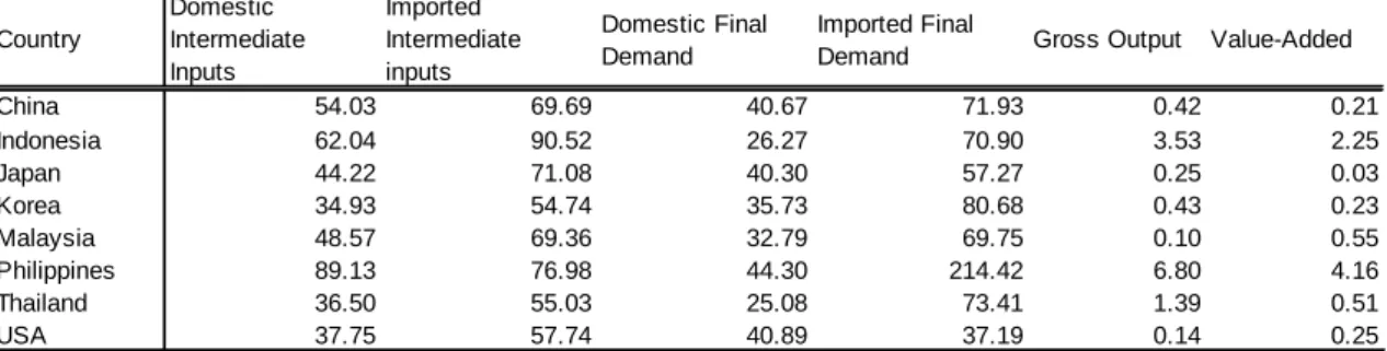
The calculated values of the six types of MAPD mentioned above are shown in Table 2. Notice that the differences in the gross output and value-added are much less significant than those in the intermediate inputs and final demand. This suggests that the adjustments

14

in the reconciliation process have mainly been made in the parts of intermediate and final demand transactions, utilizing information on the gross output or value-added, taken from the national I-O tables in many cases, as the so called "control total," which will not change and regulates magnitudes of changes in the adjustment procedure.

In general, relatively large differences are found in Indonesia and the Philippines. As seen in the previous section, the variances among the four tables tend to be large for the Philippines especially in the trade part. It is shown up as the values greater than 100% in the imported final demand for the Philippines. Despite these large discrepancies in the imported final demand, deviations are relatively larger for intermediate inputs than for final demand.

It may be because the RAS method used in the compilation process of the IDE table mainly adjusts the intermediate transactions.

Another point is that the discrepancies between imported transactions are relatively larger than those between domestic, as suggested by Jones et al. (2014). This is because the number of matrices for imported items increase as the number of countries grows. Thus, the adjustment margins in the imported items as a whole become much larger than those in the domestic transactions.

15

Table 2: Mean Absolute Percentage Differences between MRIO Tables

5. Differences in the Trade in Value-Added Indicators

In this section, we compare the IDE, ADB, OECD, and GTAP tables based on the two kinds of trade in value-added (TiVA) indicators estimated with the four MRIO data. The two kinds of TiVA indices are the ratios of domestic and imported value-added exports (VAX) to gross exports by country and industry. Let us call the former VAX related to the domestic value-added as VAXD, whereas the latter related to the imported as VAXM.VAXD of a country measure to what extent the domestic value-added is embodied in the export demand for a commodity (Johnson and Noguera 2012; Timmer et al. 2015). In a similar manner, VAXM measure the value-added imported from foreign countries.

Mean Absolute Percentage Differences between IDE and ADB Country

Domestic Intermediate Inputs

Imported Intermediate inputs

Domestic Final Demand

Imported Final

Demand Gross Output Value-Added

China 54.03 69.69 40.67 71.93 0.42 0.21

Indonesia 62.04 90.52 26.27 70.90 3.53 2.25

Japan 44.22 71.08 40.30 57.27 0.25 0.03

Korea 34.93 54.74 35.73 80.68 0.43 0.23

Malaysia 48.57 69.36 32.79 69.75 0.10 0.55

Philippines 89.13 76.98 44.30 214.42 6.80 4.16

Thailand 36.50 55.03 25.08 73.41 1.39 0.51

USA 37.75 57.74 40.89 37.19 0.14 0.25

Mean Absolute Percentage Differences between IDE and OECD Country

Domestic Intermediate Inputs

Imported Intermediate inputs

Domestic Final Demand

Imported Final

Demand Gross Output Value-Added

China 54.09 89.76 28.24 79.69 0.43 0.23

Indonesia 52.18 82.57 27.61 93.90 3.41 2.086

Japan 49.54 70.55 36.91 67.64 0.32 0.120

Korea 36.57 60.56 31.73 76.27 0.44 0.159

Malaysia 80.28 79.99 58.82 81.57 1.01 2.138

Philippines 82.72 74.42 38.08 161.61 7.27 4.162

Thailand 64.07 86.42 31.93 90.48 1.15 0.080

USA 45.63 74.83 36.41 52.47 0.21 0.193

Mean Absolute Percentage Differences between IDE and GTAP Country

Domestic Intermediate Inputs

Imported Intermediate inputs

Domestic Final Demand

Imported Final

Demand Gross Output Value-Added

China 46.13 91.75 32.90 53.96 0.89 1.29

Indonesia 65.94 94.91 28.41 70.46 3.14 3.54

Japan 36.32 91.31 33.80 37.71 0.19 0.14

Korea 41.43 83.98 43.07 55.55 0.60 0.68

Malaysia 34.03 81.27 43.74 48.34 0.40 0.15

Philippines 79.52 99.76 35.78 121.18 7.72 6.22

Thailand 41.70 79.95 35.86 59.00 1.96 2.78

USA 54.98 94.89 39.86 35.04 0.31 0.08

16

5.1 Domestic Value-Added Content of Gross Export by Country and Industry

The 𝑖𝑟 vector D of the VAXD can be derived by D=VB^dE,

where

V is a 𝑖𝑟×𝑗𝑠 diagonal matrix of the value-added to gross output ratios 𝐷_𝑖𝑠⁄𝑋_𝑖𝑠, B^d is a 𝑖𝑟×𝑗𝑠 block diagonal matrix 𝐵𝑖𝑖𝑖𝑠(𝑖=𝑠) extracted from the Leontief

inverse 𝐵_{𝑖𝑖𝑖𝑠} of the intermediate input coefficients 𝐴_{𝑖𝑖𝑖𝑠}, and

E is a 𝑖𝑟 vector of the gross export which includes both intermediate and final demand.

Then, VAXD ratio is obtained by D/E.

Figure 3(a) and (b) depicts VAXD ratios by country both for the entire activities and for the motor vehicles and motorcycles manufacturers, respectively. In relation to the entire activities, the four MRIO tables report similar ratios except the Philippines. The largest discrepancy is recorded by the ADB table, while the IDE and GTAP tables consistently present similar results. In turn, the IDE table yields comparatively different results if we focus on a specific production sector, motor vehicles and motorcycles, especially in China, Indonesia, Malaysia, and the US. In this case, the ADB and OECD tables give similar results.

17

Figure 3(a): Differences between MRIO Tables in VAXD Ratio Estimates 2004/2005 by Country

Figure 3(b): Differences between MRIO Tables in VAXD Ratio Estimates of Motor Vehicles and Motorcycles 2004/2005,

18

5.2 Imported Value-Added Content of Gross Export by Country and Industry

Analogous to the VAXD ratio, the 𝑖𝑟 vector M of the VAXM can be derived by M=VB^mE,

where

B^m is a 𝑖𝑟×𝑗𝑠 block off-diagonal matrix 𝐵𝑖𝑖𝑖𝑠(𝑖≠𝑠) extracted from the Leontief inverse 𝐵_{𝑖𝑖𝑖𝑠} of the intermediate input coefficients 𝐴_{𝑖𝑖𝑖𝑠}.

Then, VAXM ratio is obtained by M/E.

In this subsection, we mainly examine VAXM (Figure 3(c) and (d)). As for the entire activities, the ADB and GTAP tables consistently present similar results. On the other hand, the IDE and OECD table respectively give totally different VAXM ratios for the Philippines.

If we focus on the motor vehicles and motorcycles, the IDE table yields comparatively different results as in the case of VAXD, while the ADB and OECD tables consistently yield similar results. The IDE table presents the highest score for Indonesia again for motor vehicle industries. Considering the VAXD and VAXM ratios for motor vehicles and motorcycles, the IDE table potentially overvalues the value-added content of the Indonesian exports.

19

Figure 3(c): Differences between MRIO Tables in VAXM Ratio Estimates 2004/2005 by Country

Figure 3(c): Differences between MRIO Tables in VAXM Ratio Estimates 2004/2005, Motor Vehicles and Motorcycles

20

6. Concluding Remarks

This paper introduces the existing multiregional Input-Output (MRIO) Tables i.e., IDE, ADB, OECD, and GTAP with special attention to the method of constructing import matrix.

We find that each of the MRIO tables makes the import matrix in a very similar manner, i.e., using import proportionality assumption or BEC concordance with trade statistics with HS6 digit level, but IDE table. IDE conduct surveys on import demand and utilize its result for adjusting the import matrix.

This paper studies the similarities and differences among the four MRIO tables, setting the IDE table as the benchmark. The four MRIO tables are compared with respect to major economic indicators. Also, mean absolute percentage errors and TiVA indicators are estimated to make comparison of each MRIO. From the results of comparison of major economic indicators with WDI, IDE and OECD shows similarity to WDI, compared to GTAP and ADB. However, TiVA indicators show considerably different values in motor vehicles and motorcycles in Indonesia. Whereas there is some possibilities Indonesia’s TiVA is overestimation, the IDE table captures the proper production structure. In order to understand the reason why different value in the IDE table occurs, an additional survey on import demand might be required.

References

Aguir A., B. Narayanan, and R. McDougall (2016), "An Overview of the GTAP 9 Data Base." Journal of Global Economic Analysis 1(1), pp. 181-208.

Andrew R. M, G. P. Peters (2013), "A Multi-region Input-Output Table based on the Global Trade Analysis Project Database (GTAP-MRIO)," Economic Systems Research 25(1), pp. 99-121.

Baldwin R. and J. Lopez-Gonzalez (2015), "Supply-chain Trade: A Portrait of Global Patterns and Several Testable Hypotheses," The World Economy, 38(11), pp.

1682-1721.

IDE-JETRO (2013), Asian International Input-Output Table 2005, I.D.E. Statistical Data Series, No. 98. IDE-JETRO.

IDE-JETRO (2006), Asian International Input-Output Table 2000 Volume 1. Explanatory Notes, I.D.E. Statistical Data Series, No. 89. IDE-JETRO

Isard, W. (1951), "Interregional and Regional Input-Output Analysis: A Model of a